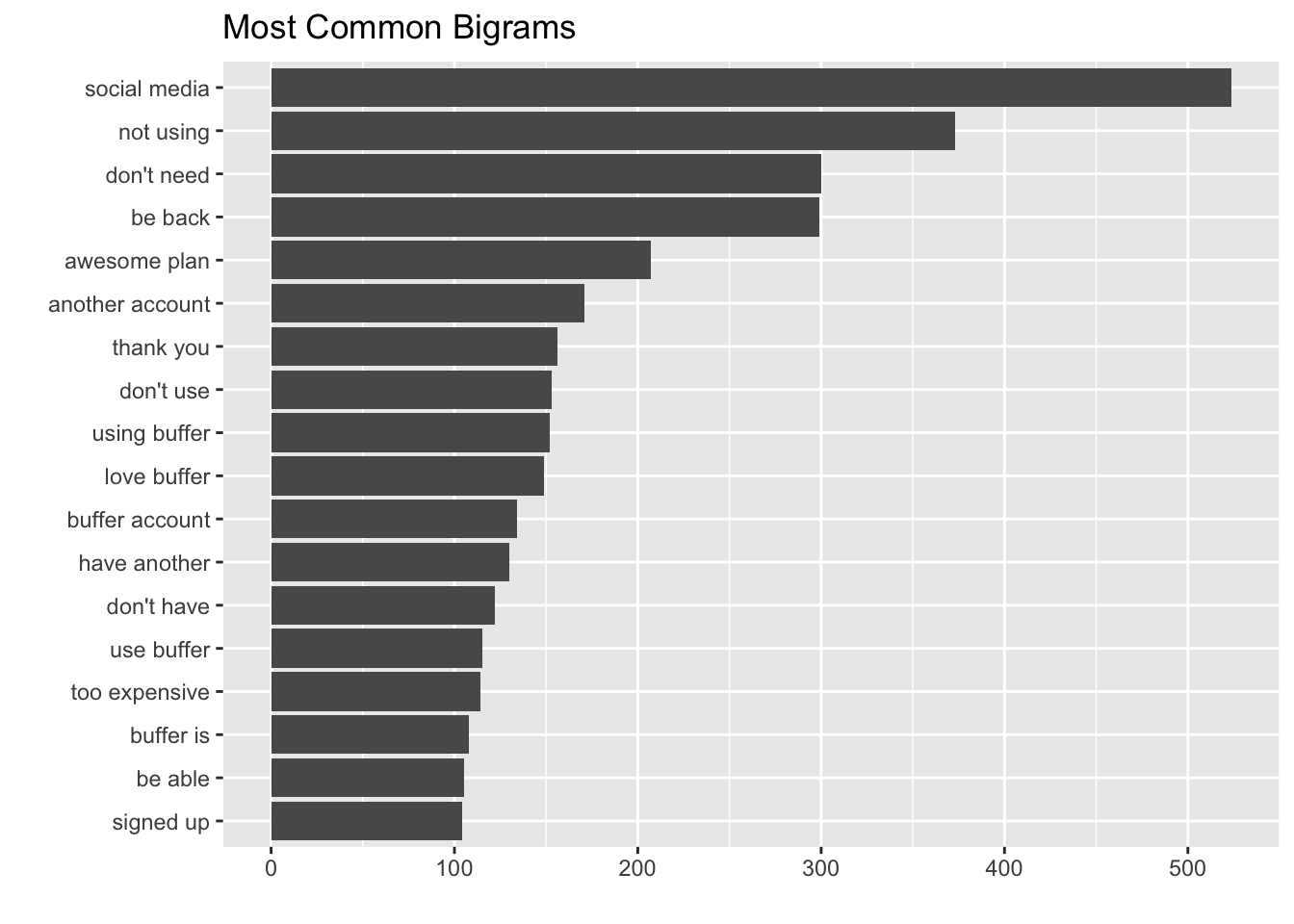
In a text analysis of churn surveys, we found that the most common reason users give for leaving Buffer is that they weren’t using it. The graph below shows the most frequently occuring pairs of words in the surveys – notice “not using” and “don’t need” at the top.
In this analysis, we’ll identify Business customers that have stopped using Buffer or use it less than they previously had. We’ll create a natural experiment in which users exposed to the experimental and control conditions are determined by their own actions. In other words, we’ll identify paying customers that stop using Buffer, or use Buffer at a decreasing rate, and compare them to paying customers with more consistent usage.
It’s a simple idea: users that stop using the product are more likely to churn. We’ve tried to predict churn before with complex models with machine learning methods, but I have high hopes for this simple approach.
How can we tell that users have stopped using Buffer? We have to define the term use first – for Buffer, the core value proposition is saving time by scheduling social media posts. Performing this function is the best proxy we have for getting value from Buffer, in my opinion.
To find users that are getting no, or less, value out of Buffer, we will look at ther frequency at which Business customers schedule social media posts. We’ll use general linear models to identify users whose usage is increasing or decreasing the quickest over time.
To begin, let’s collect all of the updates scheduled by current Business customers.
Data collection
The following SQL query returns the number of updates that every Business customer has scheduled in each week that he or she scheduled any updates.
select
  up.user_id
  , date_trunc('week', u.created_at) as user_created_at
  , date_trunc('week', up.date) as update_week
  , count(distinct up.id) as update_count
from updates as up
left join profiles as p
  on p.profile_id = up.profile_id
left join users as u
  on p.user_id = u.user_id
where up.date >= (current_date - 180)
  and up.status <> 'service'
  and u.billing_plan != 'individual'
  and u.billing_plan != 'awesome'
  and u.billing_plan != 'new_awesome'
  and u.billing_plan != '1'
  and u.billing_plan is not null
group by 1, 2, 3
Users that are on Buffer for Business trials are considered to be Business users in this query, so we’ll want to filter this dataset to include only business users that have at least one successful charge for a business subscription. The following query will give us the number of successful charges for each user, as well as the most recent subscription_id.
with recent_charges as ( -- get most recent charge ID for each customer
    select
        *
        , last_value(id) over(partition by customer order by created rows between unbounded preceding and unbounded following) as last_charge
    from stripe._charges
    where captured = TRUE
    ), last_charge as ( -- get data from only last successful charge
    select
        *
    from recent_charges
    where last_charge = id
    ) -- get info on the last subscription with a successful charge
    select
        c.created
        , c.id as charge_id
        , c.invoice
        , c.customer as customer_id
        , u.user_id
        , c.captured
        , i.subscription_id
        , s.*
        , p.interval
    from last_charge as c
    left join users as u
      on u.billing_stripe_id = c.customer
    left join stripe._invoices as i
        on c.invoice = i.id
    left join stripe._subscriptions as s
        on i.subscription_id = s.id
    left join stripe._plans as p
      on s.plan_id = p.id
  where c.created >= (current_date - 365)
    and s.status = 'active'
    and lower(s.plan_id) not like '%awesome%'
    and lower(s.plan_id) not like '%pro%'
    and lower(s.plan_id) not like '%respond%'
    and lower(s.plan_id) not like '%studio%'
    and lower(s.plan_id) not like '%lite%'
    and lower(s.plan_id) not like '%solo%'
    and lower(s.plan_id) not like '%plus%'
    and lower(s.plan_id) != 'small-29'
    and lower(s.plan_id) != 'small-149'
Now we join the two datasets with an inner_join, so that only users with successful charges are included.
# join charges and updates data
users <- biz_users %>%
  inner_join(biz_charges, by = 'user_id')

# set dates as dates
users$user_created_at <- as.Date(users$user_created_at, format = '%Y-%m-%d')
users$update_week <- as.Date(users$update_week, format = '%Y-%m-%d')

# remove unneeded datasets
rm(biz_users); rm(biz_charges)
Data tidying
Now we have an interesting problem. We have the number of updates that each Business customer send in weeks that he or she schedule any updates, but we don’t have any information on the weeks in which they didn’t sschdule any updates. We need to fill the dataset so that each user has a value for each week, even if it’s zero.
Luckily for us, the complete() function in the tidyr package is made for exactly that purpose. We will add a couple more filters, to exclude the current week (which is not yet over) and to exclude weeks that came before the user signed up for Buffer
# complete the data frame
users_complete <- users %>%
  filter(update_week != max(users$update_week)) %>%
  complete(user_id, update_week, fill = list(update_count = 0)) %>%
  select(user_id, update_week, update_count) %>%
  left_join(select(users, c(user_id, user_created_at)), by = 'user_id') %>%
  filter(update_week >= user_created_at)
Great, now we have a tidy data frame that contains the number of updates that each Business customer sent each week. In order to calculate the rate at which users’ usage is changing over time, we’ll need a bit more information. First, we add columns to the data frame for the total number updates scheduled by each person. We can then filter() to only keep users that have scheduled updates in at least 3 weeks.
We will also add a column for the total number of updates scheduled by each user.
# get year value
users_complete <- users_complete %>%
  mutate(year = year(update_week) + yday(update_week) / 365)

# get the overall update totals and number of weeksfor each user
update_totals <- users_complete %>%
  group_by(user_id) %>%
  summarize(update_total = sum(update_count),
            number_of_weeks = n_distinct(update_week[update_count > 0])) %>%
  filter(number_of_weeks >= 3)

# count the updates by week
update_week_counts <- users_complete %>%
  inner_join(update_totals, by = 'user_id') %>%
  filter(update_week != max(users$update_week))

update_week_counts
## # A tibble: 2,569,253 x 7
## user_id update_week update_count user_created_at
## <chr> <date> <dbl> <date>
## 1 000000000000000000000661 2017-02-13 0 2011-02-14
## 2 000000000000000000000661 2017-02-13 0 2011-02-14
## 3 000000000000000000000661 2017-02-13 0 2011-02-14
## 4 000000000000000000000661 2017-02-13 0 2011-02-14
## 5 000000000000000000000661 2017-02-13 0 2011-02-14
## 6 000000000000000000000661 2017-02-13 0 2011-02-14
## 7 000000000000000000000661 2017-02-13 0 2011-02-14
## 8 000000000000000000000661 2017-02-13 0 2011-02-14
## 9 000000000000000000000661 2017-02-13 0 2011-02-14
## 10 000000000000000000000661 2017-02-13 0 2011-02-14
## # ... with 2,569,243 more rows, and 3 more variables: year <dbl>,
## # update_total <dbl>, number_of_weeks <int>Using general linear models
We can think about this modeling technique answering questions like: “did a given user schedule any updates in a given week? Yes or no? How does the count of updates depend on time?”
The specific technique we’ll use is this:
Use the
nest()function to make a data frame with a list column that contains little miniature data frames for each user.Use the
map()function to apply our modeling procedure to each of those little data frames inside our big data frame.This is count data so let’s use
glm()withfamily = "binomial"for modeling.We’ll pull out the slopes and p-values from each of these models. We are comparing many slopes here and some of them are not statistically significant, so let’s apply an adjustment to the p-values for multiple comparisons.
Let’s fit the models.
# create logistic regression model
mod <- ~ glm(cbind(update_count, update_total) ~ year, ., family = "binomial")

# calculate growth rates for each user (this might take a while)
slopes <- update_week_counts %>%
  nest(-user_id) %>%
  mutate(model = map(data, mod)) %>%
  unnest(map(model, tidy)) %>%
  filter(term == "year") %>%
  arrange(desc(estimate))

slopes %>% arrange(estimate)
## # A tibble: 5,221 x 6
## user_id term estimate std.error statistic
## <chr> <chr> <dbl> <dbl> <dbl>
## 1 5975dfd5e2a81d325d08ec34 year -104.17224 6.068335 -17.16653
## 2 59649924a73330287bb13cd0 year -92.91866 3.845155 -24.16513
## 3 58dd14e3e84fe7ca6de31ad6 year -67.27158 6.535983 -10.29250
## 4 596457f51908cd0f7f34bc69 year -60.91291 5.715369 -10.65774
## 5 58e55331d842957a4d0ea6bf year -54.06255 4.071159 -13.27940
## 6 5965f441afabd391594784a7 year -53.55497 5.040584 -10.62475
## 7 58dcf362df84518a535e4525 year -51.14843 3.436332 -14.88460
## 8 593e6533840f273826cefb5a year -48.93469 3.776747 -12.95684
## 9 58bd4144ba0df71c4e428f0f year -46.07733 4.502721 -10.23322
## 10 595e8033a733302878dd3dd4 year -41.09321 1.215687 -33.80246
## # ... with 5,211 more rows, and 1 more variables: p.value <dbl>We’re finding out how influential the “time” factor is to the number of updates scheudled over time. If the slope is negative and large in magnitude, it suggests that update counts decrease significantly over time. Let’s plot the 12 users with the largest negative model estimates.
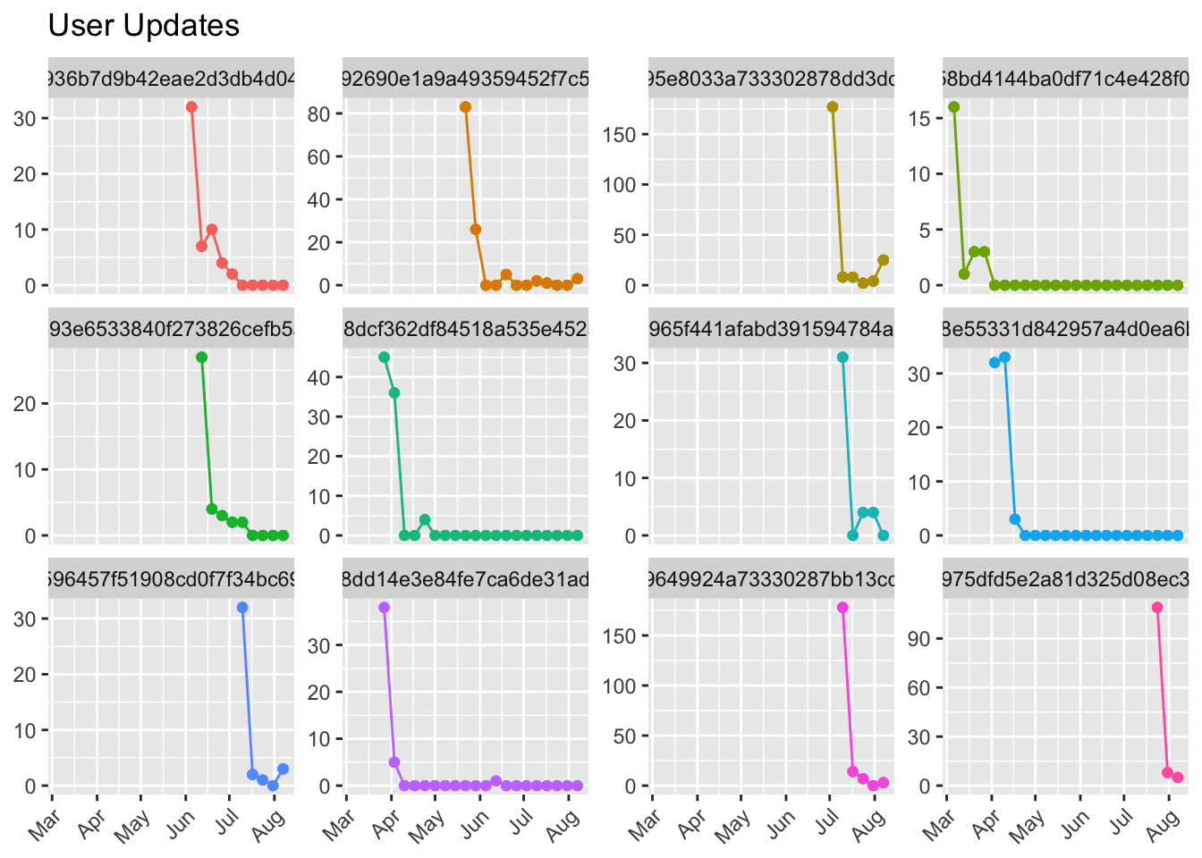
We can see that each of these users have experienced quite a dramatic drop in the number of updates scheduled over time. Let’s look at the 12 users with the largest positive estimates.
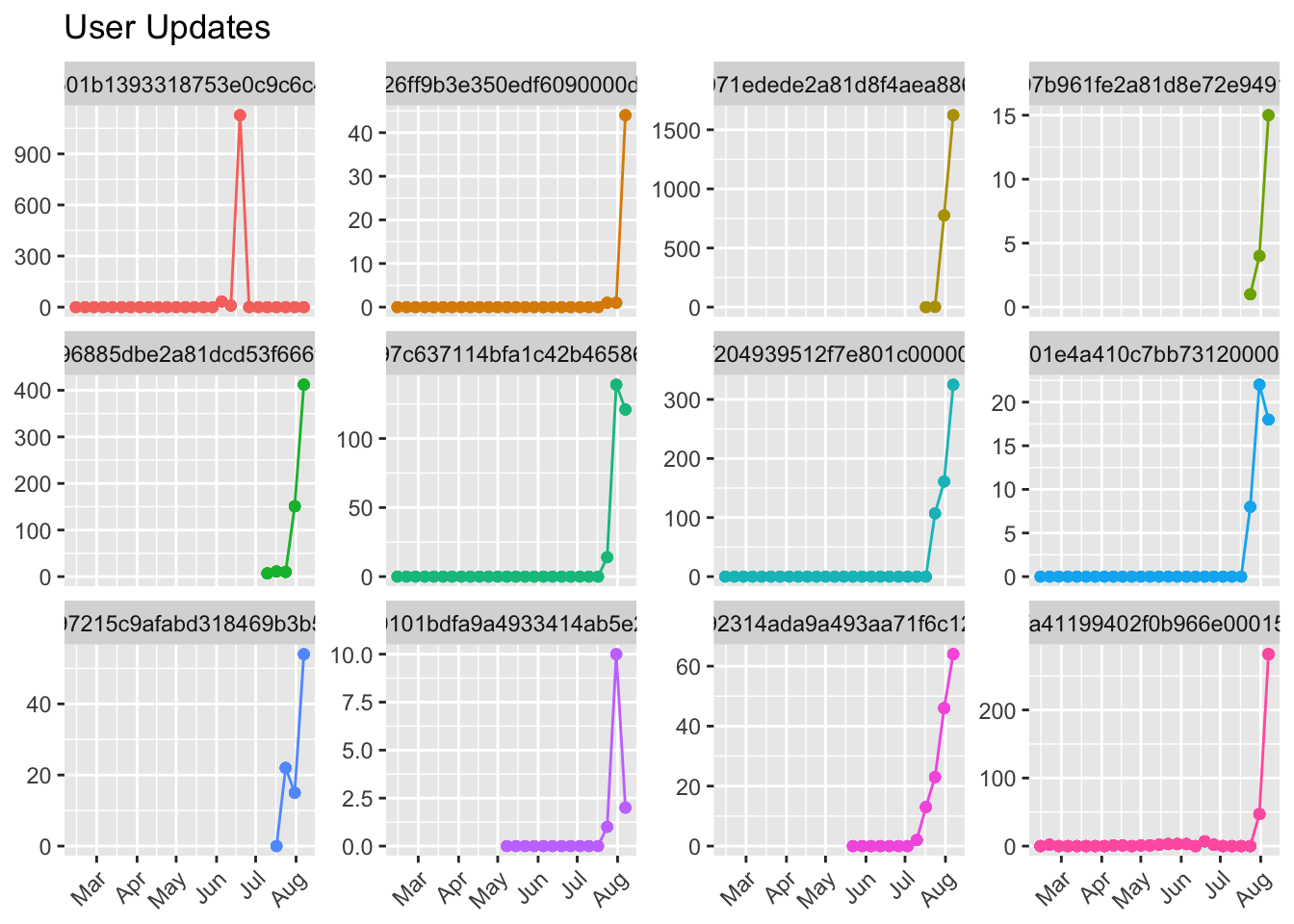
Each of these users saw a dramatic increase in the number of updates scheduled at some point. Notice the single user that scheduled 1000+ updates in a single week, and none in the next. We’ll want to filter users like that out.
Now, let’s look at users that have the smallest model estimates in terms of magnitude. These should represent users with more consistent updating habits.

Just like we thought!
Hypothesis
My hypothesis is that the users with the lowest model estimates (estimate <= - 5 and p.value <= 0.05) – those who have seen the number of updates scheduled decrease the quickest – are more likely to churn in the next two months than users with estimates greater than or equal to zero.
To test this hypothesis, I’ll gather all of those users (there are 717 of them) and monitor their churn rates over the next 60 days. I will compare these to the churn rates of the rest of the users, which will act as a control group.
slopes %>%
  filter(p.value < 0.05 & estimate <= -5) %>%
  arrange(estimate)
## # A tibble: 537 x 6
## user_id term estimate std.error statistic
## <chr> <chr> <dbl> <dbl> <dbl>
## 1 5975dfd5e2a81d325d08ec34 year -104.17224 6.068335 -17.16653
## 2 59649924a73330287bb13cd0 year -92.91866 3.845155 -24.16513
## 3 58dd14e3e84fe7ca6de31ad6 year -67.27158 6.535983 -10.29250
## 4 596457f51908cd0f7f34bc69 year -60.91291 5.715369 -10.65774
## 5 58e55331d842957a4d0ea6bf year -54.06255 4.071159 -13.27940
## 6 5965f441afabd391594784a7 year -53.55497 5.040584 -10.62475
## 7 58dcf362df84518a535e4525 year -51.14843 3.436332 -14.88460
## 8 593e6533840f273826cefb5a year -48.93469 3.776747 -12.95684
## 9 58bd4144ba0df71c4e428f0f year -46.07733 4.502721 -10.23322
## 10 595e8033a733302878dd3dd4 year -41.09321 1.215687 -33.80246
## # ... with 527 more rows, and 1 more variables: p.value <dbl>Now let’s assign users to experiment groups, based on their slope estimates.
# get user and subscription attributes
user_facts <- users %>%
  select(user_id, charge_id:interval) %>%
  unique()

# join user facts to slopes
slopes <- slopes %>%
  left_join(user_facts, by = 'user_id')

# assign treatment group
treatment_group <- slopes %>%
  filter(p.value < 0.05 & estimate <= -5)

# assign control group
control_group <- slopes %>%
  anti_join(treatment_group, by = "user_id")

# save both groups
saveRDS(treatment_group, file = 'treatment.rds')
saveRDS(control_group, file = 'control.rds')
Questions and assumptions
There are numerous small decisions made in this analysis that can have an effect on the outcome. Let’s go through them and address some questions that should be asked of the analyst.
Why filter out users with less than 3 weeks of updates? This is a very valid question. I can easily see a case in which a Business customer signs up, schedules updates for a week or two, decides Buffer isn’t right, and churns. In fact, we know that the first month is the riskiest for churn, so we’re leaving out a lot of churn candidates from the off.
It was a tricky decision, but in the end I decided to only look at Business customers with at least 3 weeks of updates so that the general linear models would have a sufficient amount of data to work with. You can imagine that it would be difficult to fit any type of model to a dataset with only two observations. We might want a 3rd observation to gather evidence of some sort of trend. It’s impossible with only one observation (this would be the case for users that have only sent updates on one week). It makes the graphs look pretty, and helps the model work well.
This is one assumption I would love to revisit and relax a bit. I think we can change it to three weeks, or perhaps even two, without much cost.
If it’s a natural experiment, why not look at users in the past? This is also a completely fair question. We should be able to apply these exact same techniques on historical data and view the outcomes, without having to wait for 60 days. I didn’t do that because 1) it’s difficult to find what plan a user had on a given date, but it’s easy to find for the current date. This is a very common problem that we should find a solution for, but I took the easy route.
This also opens up the option of designing another experiment in which we intervene on one, or both groups, to see if the intervention (an email) affects the churn rate.
That’s it for now! Please share any thoughts, comments, or questions!