When do customers churn?

Data collection

We can run the following query in Stripe Sigma to gather data on all Stripe subscriptions that have had successful charges.

select 
    subscriptions.id
  , subscriptions.created
  , subscriptions.canceled_at
  , subscriptions.plan_id
  , plans.interval
  , subscriptions.customer_id
  , count(distinct charges.id) as successful_charges
from subscriptions
left join invoices
    on invoices.subscription_id = subscriptions.id
left join charges
    on charges.invoice_id = invoices.id
left join plans
    on plans.id = subscriptions.plan_id
where charges.paid = TRUE
group by 1, 2, 3, 4, 5, 6

I exported this data to a CSV, which we’ll read into R now.

# Read CSV
subs <- read.csv("~/Downloads/subscriptions.csv", header = T)

There are over 185 thousand subscriptions in this dataset. We include the subscription ID, when it was created, the cancellation date (if it was cancelled), the plan ID, the billing interval, the customer ID, and the number of successful charges.

Let’s calculate a new variable, the length of the subscription in days. We also need to create an indicator variable to let us know if the subscription has churned.

# Calculate subscription length and churn indicator
subs <- subs %>%
  mutate(length = as.numeric(canceled_at - created),
         did_churn = ifelse(is.na(canceled_at), 0, 1))

Survival analysis

To get a better understanding of exactly when customers churn, we’ll use a technique called survival analysis. Clasically, survival analysis was used to model the time it takes for people to die of a disease. However it can be used to model and analyze the time it takes for a specific event to occur, churn in this case.

It is particularly useful because of missing data – there must be subscriptions that will churn in our dataset that haven’t done so yet. This is called censoring, and in particular right censoring.

Right censoring occurs when the date of the event is unknown, but is after some known date. Survival analysis can account for this kind of censoring.

There is also left censoring, for example when the date the subscription was created is unknown, but that is less applicable to our case.

The survival function, or survival curve, (S) models the probability that the time of the event (T) is greater than some specified time (t).

Let’s build the survival curve and plot it out.

# Kaplan Meier survival curve
subs$survival <- Surv(subs$length, subs$did_churn)

# Fit the model
fit <- survfit(survival ~ 1, data = subs)

# Create survival plot
ggsurvplot(fit, data = subs, risk.table = "percentage", 
           risk.table.title = "Percent Remaining",
           break.x.by = 60, xlim = c(0, 720))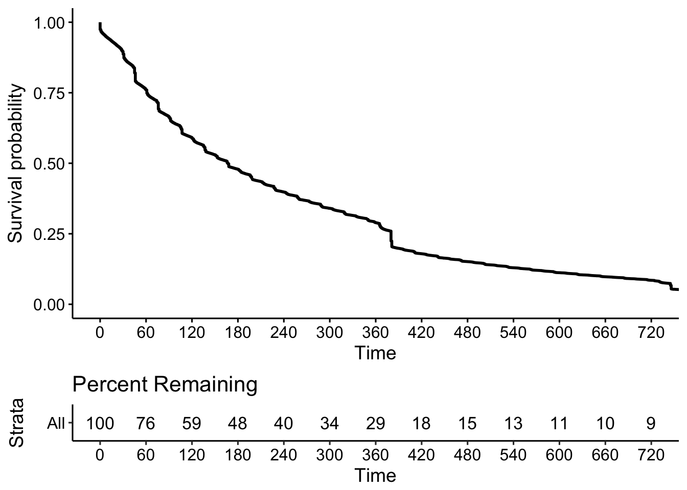

The plot shows the percent of subscriptions still active X days after creating the subscription. The risk table below the graph shows the percent of subscription still remaining after X days. We can see that there are kinks around every 30 days, as well as a large kink at 365 days, when many annual subscriptions are cancelled.

It is important to note that the curve is steeper earlier on, suggesting that larger percentages of subscriptions churn early on in their lifetimes. It might be useful to break this graph up to visualize the survival curves for both monthly and annual subscriptions.

# Fit the second model
fit2 <- survfit(survival ~ interval, data = subs)

# Create survival plot
ggsurvplot(fit2, data = subs, risk.table = "percentage", 
           risk.table.height = 0.30, surv.plot.height = 0.70,
           risk.table.y.text = FALSE, tables.y.text = FALSE,
           risk.table.title = "Percent Remaining",
           break.x.by = 60, xlim = c(0, 720))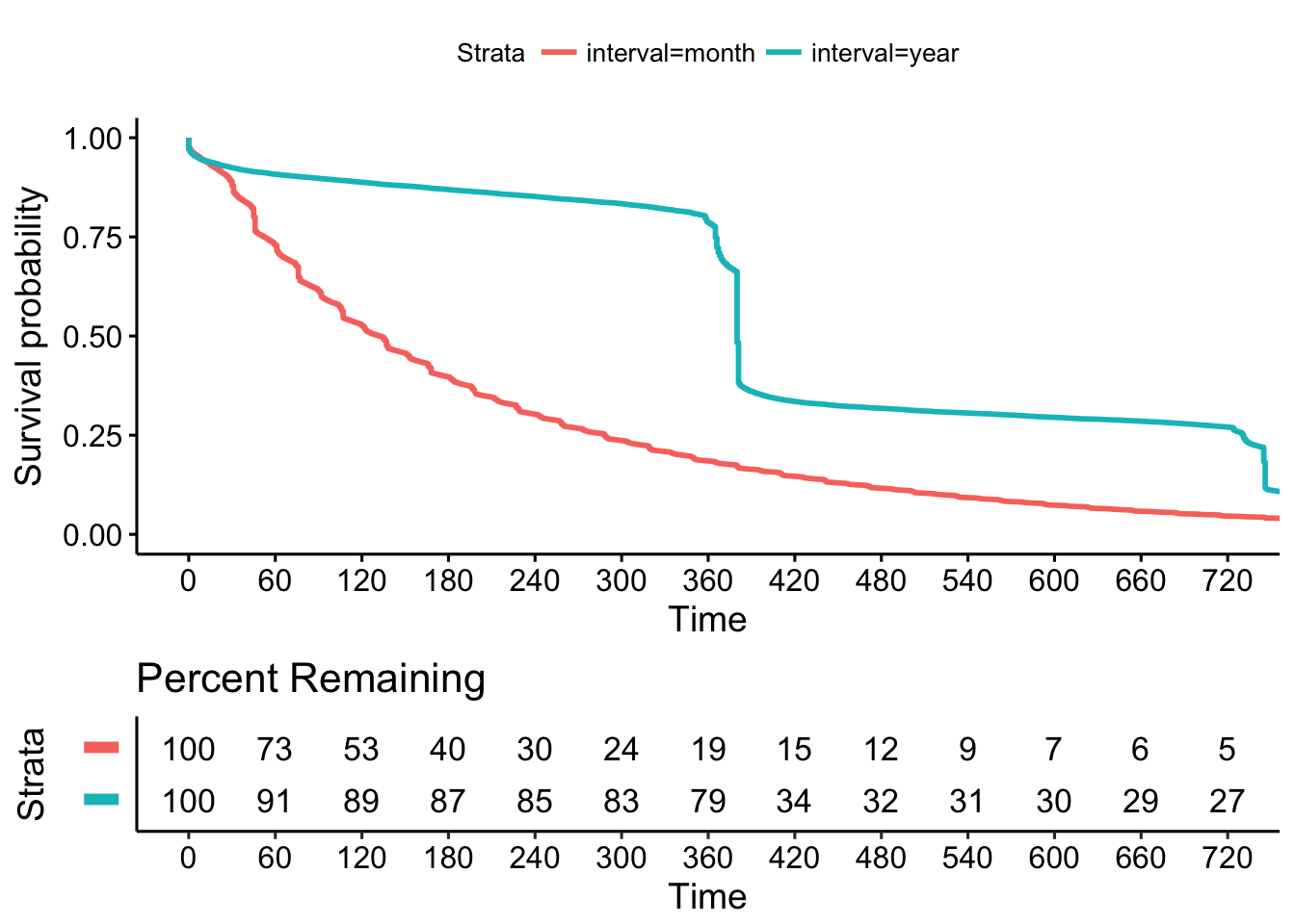

In the graph above, the survival curves have been segmented by the billing interval. By day 60, around 73% of monthly subscriptions were still active, compared to around 91% of annual subscriptions.

Annual subscriptions have a very low rate of churn, up until the 365 day mark, after which time almost 70% of annual subscriptions are churned!

V2 Business Subscriptions

Let’s get a little more granular, and look only at v2 Buffer for Business subscriptions.

# Drop survival object
subs$survival <- NULL

# Identify v2 business plans
biz_plans <- c('business_v2_agency_monthly', 'business_v2_agency_yearly', 'business_v2_business_monthly',
               'business_v2_business_yearly', 'business_v2_small_monthly', 'business_v2_small_yearly')

# Get business subscriptions
biz_subs <- subs %>%
  filter(plan_id %in% biz_plans)

Now let’s take the same approach as before, and visualize the survival curves of the annual and monthly plans.

# Kaplan Meier survival object
biz_subs$survival <- Surv(biz_subs$length, biz_subs$did_churn)

# Fit the third model
fit3 <- survfit(survival ~ interval, data = biz_subs)

# Create survival plot
ggsurvplot(fit3, data = biz_subs, risk.table = "percentage", 
           risk.table.height = 0.30, surv.plot.height = 0.70,
           risk.table.y.text = FALSE, tables.y.text = FALSE,
           risk.table.title = "Percent Remaining",
           break.x.by = 30, xlim = c(0, 420))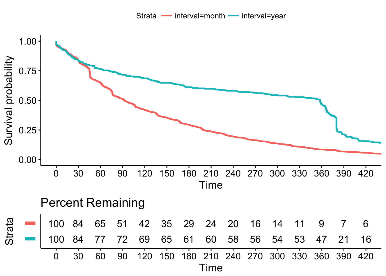

Based on the risk table, we can gather that approximately 16% of V2 Business subscriptions churn in the first 30 days.

• By day 60, only 65% of monthly subscriptions and 77% of annual subscriptions remain.
• By day 90, almost half of monthly subscriptions and around 30% of annual subscriptions have churned.
• By day 180, around 70% of monthly subscriptions and 40% of annual subscriptions have churned.
• By day 365, around 90% of monthly subscriptions and 80% of annual subscriptions have churned.

This paints a fairly worrying picture of churn for the V2 Business subscriptions. It is good to know that efforts are being made to reduce churn and make sure people get on the best plan for their needs. :)