Buffer introduced a minimum vacation policy a year ago, in which we encouraged team members to take a certain number of vacation days, at minimum. If an individual was “falling behind”, i.e. not taking as much vacation as he or she should, our team would kindly remind the individual that vacation is beneficial to the entire team’s productivity and happiness.
In this analysis we’ll try to measure the effect that this policy has had on the team in 2017. We use timetastic to schedule time off, and we’re lucky enough to have a nice report that shows how much time each team member has taken off.
Data collection
We’ll read the data in from a CSV that we exported from timetastic. I saved the data as an R data object – let’s read it into this R session.
# load data
days <- readRDS('vacation2017.rds')
Now let’s clean up the column names and set the dates as date types.
# change column names
colnames(days) <- safe_names(colnames(days))

# create function to set date as date object
set_date <- function(column) {
  column <- as.Date(column, format = '%Y-%m-%d')
}

# apply function to date columns
days[c(3, 9:11)] <- lapply(days[c(3, 9:11)], set_date)
## Warning in strptime(x, format, tz = "GMT"): unknown timezone 'default/
## America/New_York'Great! Now we need to do a bit of tidying to make the analysis easier.
Data tidying
We only want to look at time taken off in 2017, so let’s filter out dates that don’t apply. We also want to filter to only look at vacation days taken off. We also exclude people that are no longer on the team.
# filter dates
vacation <- days %>%
  filter(start_time >= '2017-01-01' & leave_type == "Vacation" & status == "Authorised") %>%
  mutate(end_time = ifelse(end_time > '2017-12-31', as.Date('2017-12-31'), end_time))
Now let’s group the data by team member, so that we can see the total number of days taken off by each.
# group by person
by_user <- vacation %>%
  group_by(user) %>%
  summarise(total_working_days = sum(working))
We’ll “bin” the number of vacation days, so that it becomes a categorical variable instead of a numeric one. This will make plotting a little easier, as we’ll be able to see the number of team members that took, say, 1 to 5 days in the past year.
# make bins for total days
cuts <- c(-Inf, seq(0, 50, 5))

# bin the days
by_user <- by_user %>%
  mutate(days_off = cut(total_working_days, cuts))
Alright, let’s make some fun plots.
Exploratory analysis
So how much time has the team taken off in the past year?
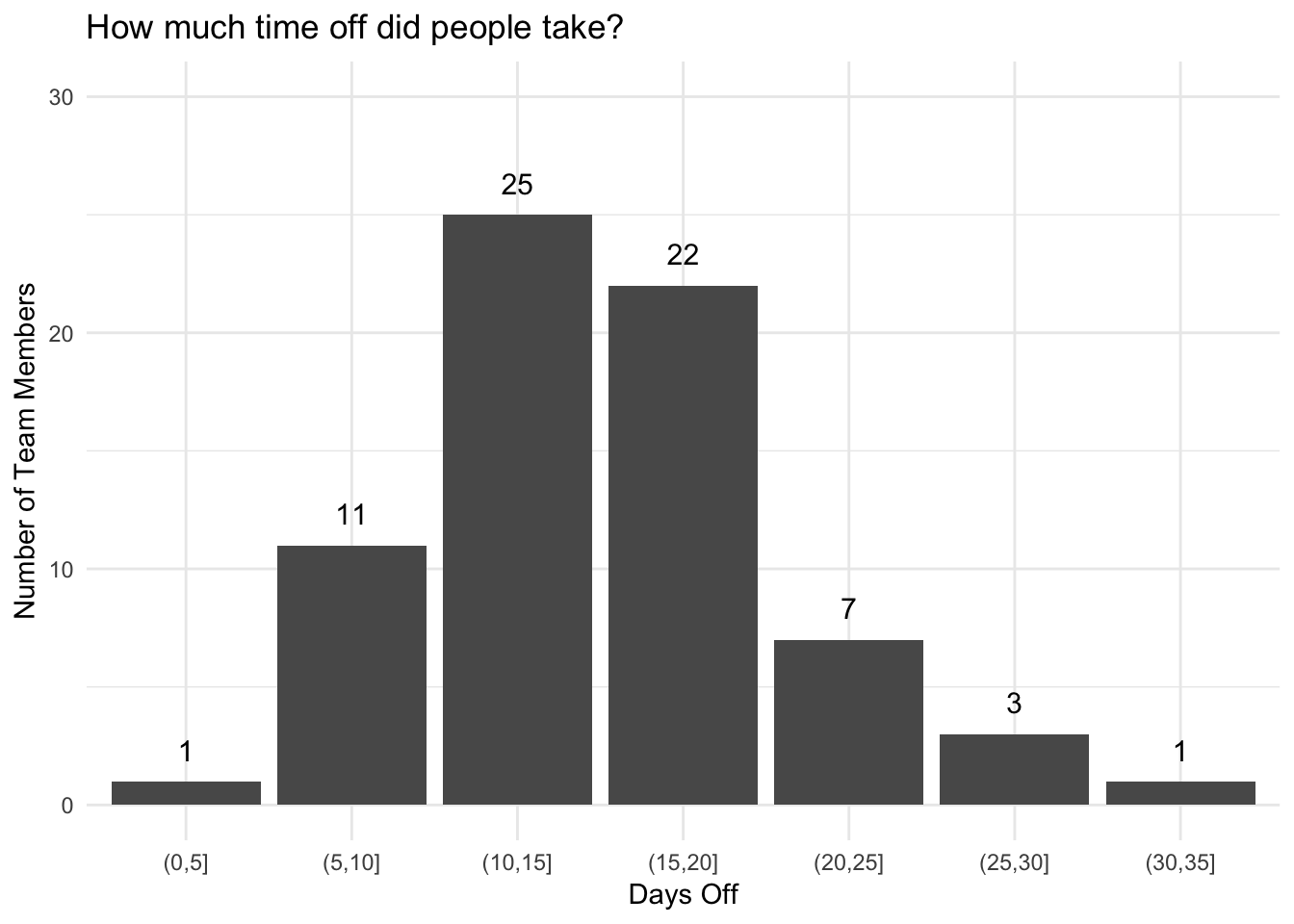
The average number of vacation days taken by Buffer employees in the past year is 18.2, and the median is 16.5. Around a quarter of the team has taken 12 or less vacation days, and another quarter has taken over 24 days off.
The plot above shows that many team members have only taken 10-15 vacation days. We have one team member who has only taken 2 days off over the past year and one who has taken over 40 days!
How does this look for people that live in different regions? Let’s look at the median number of vacation days taken by team members in each region.
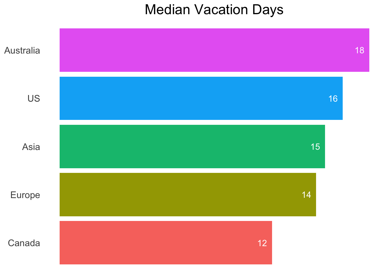
This is interesting! We haven’t yet taken into account the variance in the number of vacation days taken, so let’s visualize the distribution of vacation days taken from team members that live in each region.
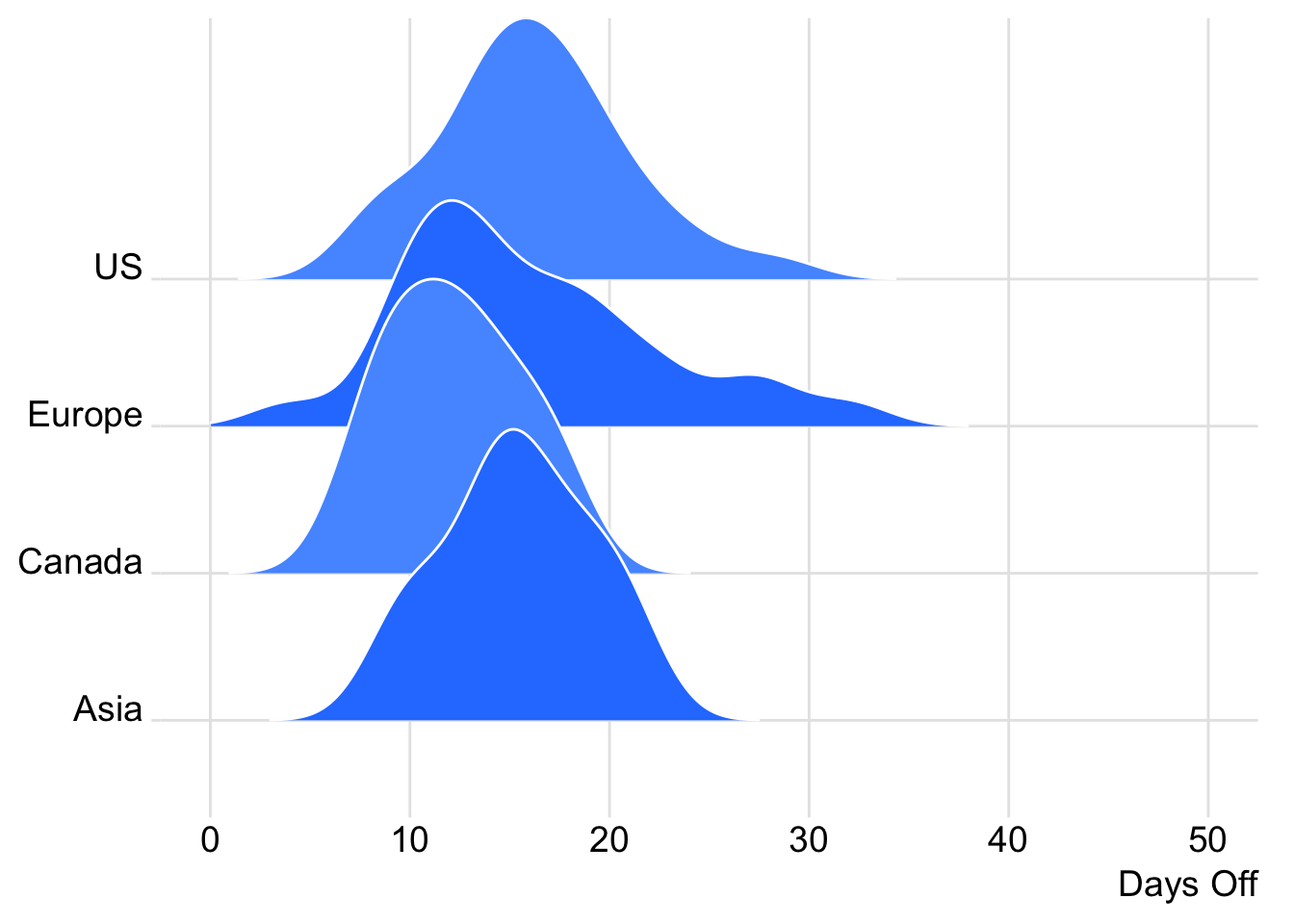
Overall, it looks like people are following the recommendations of the policy. The center of the distribution of days off for Americans is between 10 and 20, as is the center of the distribution of days off for Europeans.
The distribution is far wider for Europeans, which suggests that there are people that have taken very few days off (one person has only taken 2) and people that have taken many days off (one has taken 44.5).
Canadians seem to know how to relax. Their distribution is more uniformly distributed and is closer to the 30-40 day range.
Team members in Asia represent a smaller sample, but their distribution is centered around 11 days.
That’s it for now
That was fun! Let me know if you have any thoughts or questions!