TL;DR
Changes to the app and landing pages have led to a large (30%) and significant increase in Awesome trial starts.
There are indications of a positive effect on Awesome MRR, but the probability of a true effect is inconclusive.
The free plan experiment was a major confounding factor that did increase Awesome MRR.
Background
Back in September, Buffer experienced a period of relatively low MRR growth. This was especially impactful for the Awesome plans, which saw a sharp and distinct decrease in growth.
There were several factors that could have contributed to this change: landing page changes, product changes, churn, and bugs all conspired to create a batch effect that slowed growth for Awesome subscriptions. After a lot of analysis and many conversations, we took action on October 11 by fixing a bug that prevented the Awesome upgrade modal from appearing and on October 13 by reverting some changes made to the landing page.
It has been a few months since we’ve made these changes, so we can try to measure the impact that these changes have made so far on Awesome trials and Awesome MRR. In order to estimate the effects, we’ll use an R package written by Google engineers for causal inference called CausalImpact. A controlled experiment is the gold standard for estimating effect sizes, but we don’t have that here – we effectively put everyone in the experiment group. Sometimes that is necessary! There are still ways to estimate effect sizes.
The idea is this: given a response time series (e.g. trials, revenue) and a set of control time series (e.g. clicks in non-affected markets or clicks on other sites), the package constructs a Bayesian structural time-series model. This model is then used to try and predict the counterfactual, i.e. how the response metric would have evolved after the intervention if the intervention had never occurred.
The model assumes that the time series of the treated unit can be explained in terms of a set of covariates which were themselves not affected by the intervention whose causal effect we are interested in. We’ll use time and business trials as the covariates.
Let’s give it a shot!
Awesome trials
Before we look at MRR, let’s look at the number of Awesome trials started. I believe these are more directly under our control - we have a greater influence on the number of trial starts than we do over the number of people that subscribe or churn.
We’ll use the data in this Look and import it using the buffer package.
# import data from Looker
# trials <- get_look(4171)
Let’s do a bit of cleanup now.
# rename columns
colnames(trials) <- c('start_date', 'awesome_trials', 'business_trials')

# set dates as date type
trials$start_date <- as.Date(trials$start_date, format = '%Y-%m-%d')
## Warning in strptime(x, format, tz = "GMT"): unknown timezone 'default/
## America/New_York'Great, let’s plot these values out.
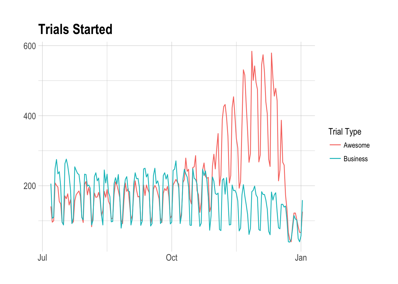
Immediately we can see a large “bump” in the number of Awesome trials around the end of October. This is likely due to an experiment that we ran to measure the effects of a simplified and more-limited free plan. This is a major confounding variable that may also effect revenue, but we may be able to control for it.
# load zoo package
library(zoo)

# create time series object
trials_ts <- zoo(dplyr::select(trials, awesome_trials:business_trials), trials$start_date)

# specify the pre and post periods
pre.period <- as.Date(c("2017-07-04", "2017-10-10"))
post.period <- as.Date(c("2017-10-11", "2017-10-27"))
We defined the post-intervention period to be from October 11, when the changes were made, to October 27. The reason that I cut it off was that the free plan experiment began around October 26, and this confounds the data. We try to limit this effect somewhat here. To perform inference, we run the analysis using the CausalImpact command.
# run analysis
impact <- CausalImpact(trials_ts, pre.period, post.period, model.args = list(niter = 5000, nseasons = 7))
Let’s plot the outcome of the model.
# plot results
plot(impact)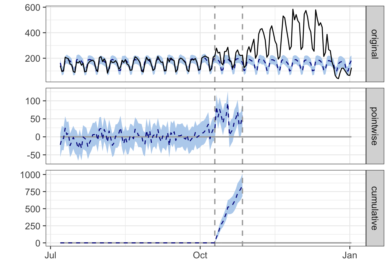
The resulting plot is quite interesting. The top panel in the graph shows the counterfactual as a dotted line and blue confidence interval – this is the estimate of what trials would have been without an intervention. The solid black line shows the number of Awesome trials that actually were started.
The middle panel shows the point estimate of the effect of the intervention on each day. We can see that the point estimate of the effect is around 25-100 extra trials each day.
The bottom panel visualizes the cumulative effect that the intervention had on Awesome trial starts. As of October 31, the cumulative effect is around 1000 extra trial starts. Wow!
How can we determine if this effect is statistically significant? That is the core question, since we don’t have a controlled experiment here.
# get summary
summary(impact)
## Posterior inference {CausalImpact}
##
## Average Cumulative
## Actual 217 3689
## Prediction (s.d.) 167 (5) 2839 (84)
## 95% CI [157, 177] [2674, 3006]
##
## Absolute effect (s.d.) 50 (5) 850 (84)
## 95% CI [40, 60] [683, 1015]
##
## Relative effect (s.d.) 30% (3%) 30% (3%)
## 95% CI [24%, 36%] [24%, 36%]
##
## Posterior tail-area probability p: 2e-04
## Posterior prob. of a causal effect: 99.97993%
##
## For more details, type: summary(impact, "report")This summary tells us that we’ve seen an average of 217 awesome trials since the action was taken. The predicted average, based on previous months worth of data, would have been 166. The relative effect was a 30% increase in awesome trial starts – the 95% confidence interval for this effect size is [24%, 36%]. That’s a big effect!
The probability of a true causal effect is very high (99.98%), which makes sense given what we saw in the graphs. Nice!
Awesome MRR
I have a hunch that this effect will be harder to detect, if it does exist. We’ll use the same approach as we did with trials, excepct this time we’ll look at Awesome MRR in this look.
# collect data
mrr <- get_look(4173)

# remove first row
mrr <- mrr[-1, ]

# rename columns
colnames(mrr) <- c('date', 'awesome_mrr', 'business_mrr')

# set numeric values
mrr$awesome_mrr <- as.numeric(as.character(mrr$awesome_mrr))
mrr$business_mrr <- as.numeric(as.character(mrr$business_mrr))

# set as date
mrr$date <- as.Date(mrr$date, format = '%Y-%m-%d')
Let’s plot the values.
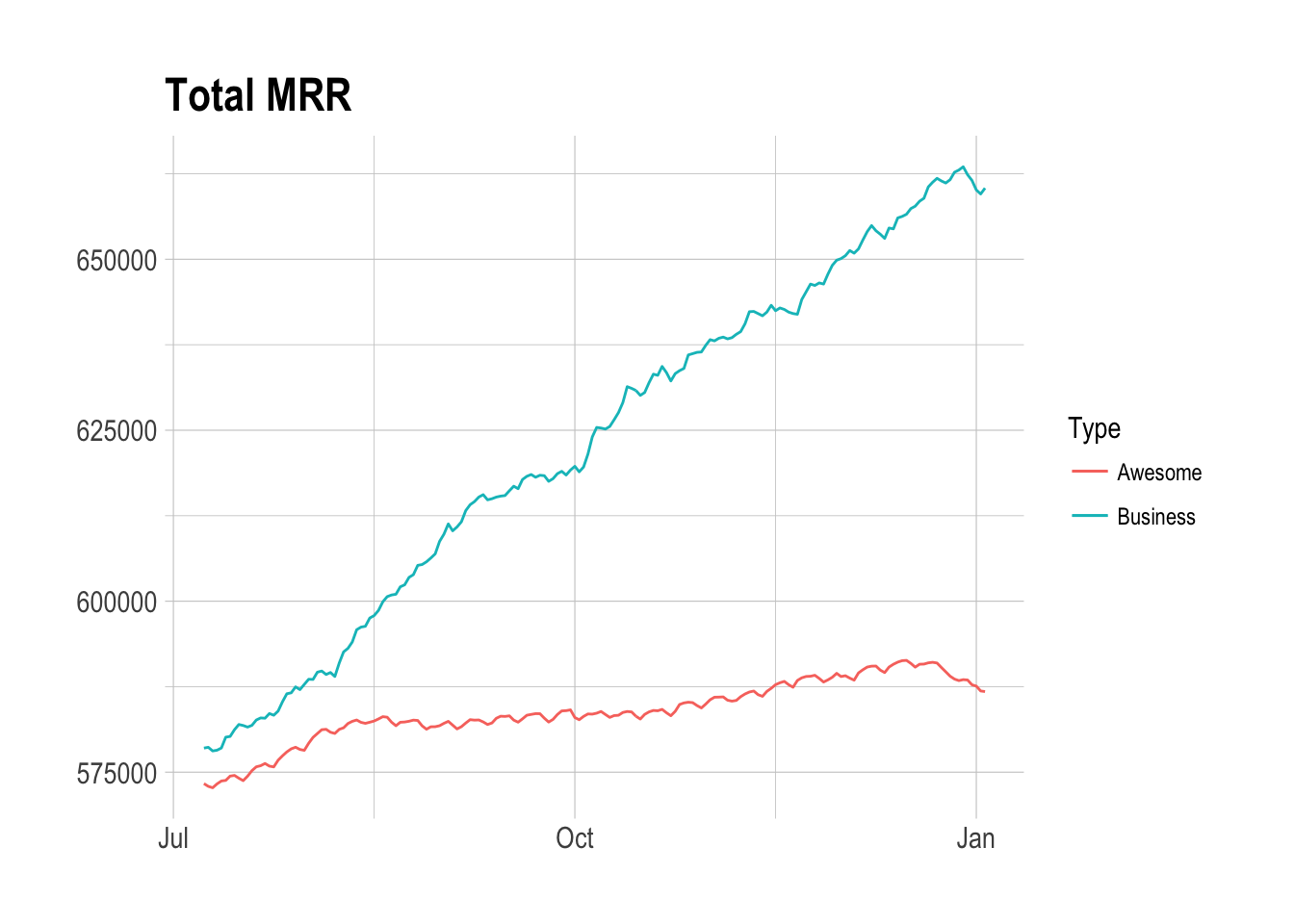
Now let’s try to see if we’ve been able to make any impact on Awesome MRR.
# create time series object
mrr_ts <- zoo(dplyr::select(mrr, awesome_mrr), mrr$date)

# specify the pre and post periods
pre.period <- as.Date(c("2017-07-05", "2017-10-10"))
post.period <- as.Date(c("2017-10-11", "2017-10-31"))

# run analysis
mrr_impact <- CausalImpact(mrr_ts, pre.period, post.period, model.args = list(niter = 5000, nseasons = 7))

# plot impact
plot(mrr_impact)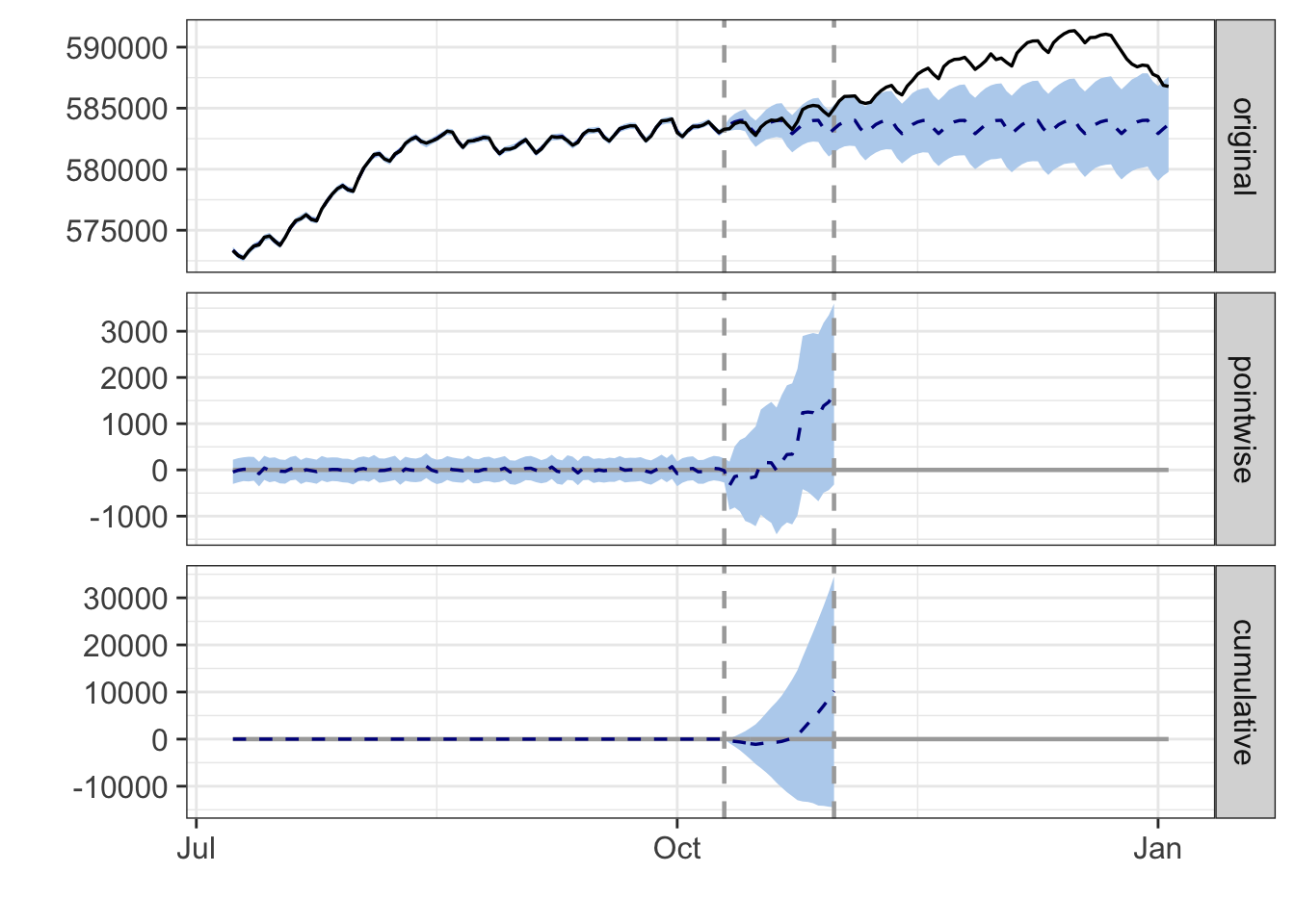
Please ignore the cumulative panel, as it is not relevant to us here (MRR is already an aggregation and we don’t sum it every day).
The original panel shows the counterfactual, as well as the confidence bands, as the dotted line and blue ribbon. The solid black line is the actual MRR amounts we’ve seen. We can see here that the observed values (the solid black line) are within the bounds of the confidence interval during the time window we have selected. However, we can see that there are indications of a positive effect on Awesome MRR during this timeframe.
If we look beyond the effect period, we can see that the free plan experiment does indeed seem to have a positive effect on Awesome MRR.
# summarise model
summary(mrr_impact)
## Posterior inference {CausalImpact}
##
## Average Cumulative
## Actual 5.8e+05 1.2e+07
## Prediction (s.d.) 5.8e+05 (596) 1.2e+07 (12517)
## 95% CI [5.8e+05, 5.8e+05] [1.2e+07, 1.2e+07]
##
## Absolute effect (s.d.) 486 (596) 10202 (12517)
## 95% CI [-689, 1643] [-14465, 34511]
##
## Relative effect (s.d.) 0.083% (0.1%) 0.083% (0.1%)
## 95% CI [-0.12%, 0.28%] [-0.12%, 0.28%]
##
## Posterior tail-area probability p: 0.20628
## Posterior prob. of a causal effect: 79%
##
## For more details, type: summary(impact, "report")The summary confirms that we have not seen a sufficiently large enough effect on Awesome MRR to attribute it directly to the changes made to landing pages.