Defining an Activation Rate

Data Collection

We’ll want to gather all users that signed up before three months ago. We don’t yet know if users that signed up in the past three months were “successful” or not. We also want to know how many profiles they added in the first week and how many updates were created. We want users that signed up between December 1, 2016 and December 1, 2017.

We’ll gather that data with the following query.

with profiles as (
  select 
    u.user_id
    , count(distinct p.id) as profiles
  from dbt.users as u
  left join dbt.profiles as p
  on u.user_id = p.user_id and datediff(day, u.created_at, p.created_at) < 7
  where u.created_at >= '2016-12-01' and u.created_at <= '2017-12-01'
  group by 1
),

last_active_date as (
  select 
    user_id
    , max(date(created_at)) as last_active_date
  from dbt.updates
  where was_sent_with_buffer
  and status != 'failed'
  and created_at > '2016-12-01'
  and client_id in (
        '5022676c169f37db0e00001c', -- API and Extension
        '4e9680c0512f7ed322000000', -- iOS App
        '4e9680b8512f7e6b22000000', -- Android App
        '5022676c169f37db0e00001c', -- Feeds
        '5022676c169f37db0e00001c', -- Power Scheduler
        '539e533c856c49c654ed5e47', -- Buffer for Mac
        '5305d8f7e4c1560b50000008'  -- Buffer Wordpress Plugin
        )
  group by 1
)

select 
  u.user_id
  , date(u.created_at) as signup_date
  , p.profiles
  , l.last_active_date
  , count(distinct up.id) as updates
  , count(distinct date(up.created_at)) as days_active
from dbt.users as u
left join dbt.updates as up
  on (u.user_id = up.user_id and datediff(day, u.created_at, up.created_at) < 7)
left join profiles as p 
  on u.user_id = p.user_id
left join last_active_date as l
  on u.user_id = l.user_id
where u.created_at >= '2016-12-01' and u.created_at <= '2017-12-01'
  and (up.was_sent_with_buffer = TRUE or up.was_sent_with_buffer is null)
  and (up.status != 'failed' or up.status is null)
  group by 1, 2, 3, 4

Great, we now have around 1.4 million Buffer users to analyze!

Data Tidying

We also want to know if the user was successful. We do this by determining if the user was still active 90 days after signing up. If the user didn’t send any updates, we’ll set their last_active_date to the signup_date value.

# set last active date
users$last_active_date[is.na(users$last_active_date)] <- users$signup_date

# determine if user was successful
users <- users %>% 
  mutate(successful = as.numeric(last_active_date - signup_date) >= 90)

Let’s see what proportion of signups were retained for three months.

# get success rate
users %>% 
  group_by(successful) %>% 
  summarise(users = n_distinct(user_id)) %>% 
  mutate(percent = users / sum(users))

## # A tibble: 2 x 3
##   successful   users percent
##   <lgl>        <int>   <dbl>
## 1 F          1028578   0.715
## 2 T           410653   0.285

Around 29% of users were retained for three months.

Searching for Activation

Now let’s see how well these metrics correlate with success. To do so, we’ll use a logistic regression model.

# define logistic regression model
mod <- glm(successful ~ profiles + updates + days_active, data = users, family = "binomial")

# summarize the model
summary(mod)

## 
## Call:
## glm(formula = successful ~ profiles + updates + days_active, 
##     family = "binomial", data = users)
## 
## Deviance Residuals: 
##     Min       1Q   Median       3Q      Max  
## -5.6509  -0.8173  -0.7784   1.4191   2.8803  
## 
## Coefficients:
##               Estimate Std. Error  z value Pr(>|z|)    
## (Intercept) -1.1041152  0.0025668 -430.157   <2e-16 ***
## profiles     0.0651174  0.0013520   48.163   <2e-16 ***
## updates     -0.0002771  0.0000295   -9.394   <2e-16 ***
## days_active  0.1143397  0.0012843   89.028   <2e-16 ***
## ---
## Signif. codes:  0 '***' 0.001 '**' 0.01 '*' 0.05 '.' 0.1 ' ' 1
## 
## (Dispersion parameter for binomial family taken to be 1)
## 
##     Null deviance: 1721077  on 1439230  degrees of freedom
## Residual deviance: 1706614  on 1439227  degrees of freedom
## AIC: 1706622
## 
## Number of Fisher Scoring iterations: 5

All three metrics seem to have very significant effects on the probability of a user being successful. Interesting, the correlation between updates and success is negative! I have a hunch that this is because of outliers, folks that send thousands of updates in their first days. Let’s remove them from the dataset.

# find quantiles for updates
quantile(users$updates, probs = c(0, 0.5, 0.99, 0.995, 0.999))

##    0%   50%   99% 99.5% 99.9% 
##     0     0    75   117   414

The 99th percentile for updates created in the first week is 75 and the 99.5th percentile is 117, so let’s remove users that created 120 or more updates in their first week.

# remove outliers
users <- filter(users, updates < 120)

Now let’s rebuild the model.

# define logistic regression model
mod <- glm(successful ~ profiles + updates + days_active, data = users, family = "binomial")

# summarize the model
summary(mod)

## 
## Call:
## glm(formula = successful ~ profiles + updates + days_active, 
##     family = "binomial", data = users)
## 
## Deviance Residuals: 
##     Min       1Q   Median       3Q      Max  
## -3.8116  -0.7995  -0.7807   1.4352   1.6600  
## 
## Coefficients:
##               Estimate Std. Error z value Pr(>|z|)    
## (Intercept) -1.0872522  0.0026230 -414.51   <2e-16 ***
## profiles     0.0552942  0.0014378   38.46   <2e-16 ***
## updates      0.0136422  0.0002267   60.18   <2e-16 ***
## days_active  0.0396148  0.0017628   22.47   <2e-16 ***
## ---
## Signif. codes:  0 '***' 0.001 '**' 0.01 '*' 0.05 '.' 0.1 ' ' 1
## 
## (Dispersion parameter for binomial family taken to be 1)
## 
##     Null deviance: 1710867  on 1432247  degrees of freedom
## Residual deviance: 1693257  on 1432244  degrees of freedom
## AIC: 1693265
## 
## Number of Fisher Scoring iterations: 4

That’s much more like it. :)

Updates

In the first activation metric, we decided that three updates in seven days was optimal. We can examine the success rate for users that sent a certain number of updates in their first week to help with this.

# define bins
cuts <- c(1, 5, 10, 20, 50, 100)

# create update bins
users <- users %>% 
  mutate(update_bin = cut(updates, breaks = cuts, include.lowest = TRUE))

# plot success rate for each bin
users %>% 
  group_by(update_bin, successful) %>% 
  summarise(users = n_distinct(user_id)) %>% 
  mutate(percent = users / sum(users)) %>% 
  filter(successful & !is.na(update_bin)) %>% 
  ggplot(aes(x = update_bin, y = percent)) +
  geom_bar(stat = 'identity') +
  theme_ipsum() +
  scale_y_continuous(labels = percent) +
  labs(x = "Updates Created in First Week", y = NULL,
       title = "Success Rate by Update Bin", 
       subtitle = "Success: Retained for 90 Days")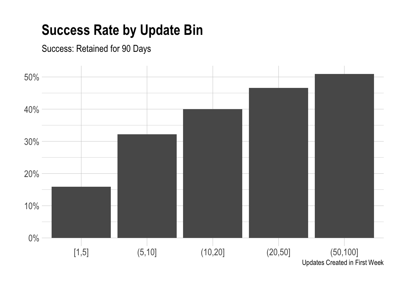

We can see that the success rate increases as the update bins increase. Over 50% of users that create 50 or more updates in their first week are retained for three months. The problem is that there are very few users that do this. We see that there is a big jump from 1 to 20 updates. Let’s zoom in there and see if there is a point with the greatest marginal return.

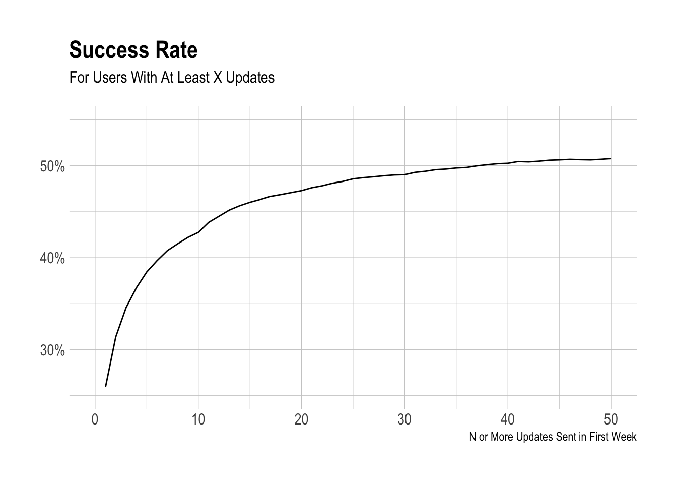
The graph below shows the proportion of users with at least X updates that were reteined for three months. We can see that there are diminishing returns, but it is tough to tell where an inflection point might be. One feature that is cool to see is the little bump at 11 updates. This exists because of the queue limit. Whene a user signs up for Buffer on a free plan, they can only have 10 updates scheduled at one time for a single profile.

What would this grpah look like if we zoomed into only look at 1-15 updates?

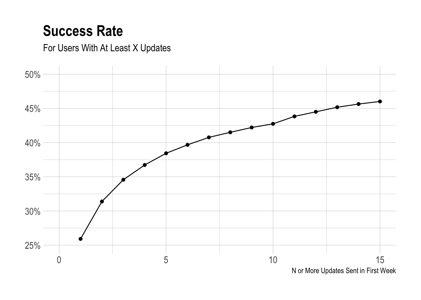
To my eyes, three updates seems as good a choice as any. There are clear diminishing returns after three updates, and a significant number of users (358 thousand) did successfully take the action.

Profiles

We’ll take the same approach to look at profiles.

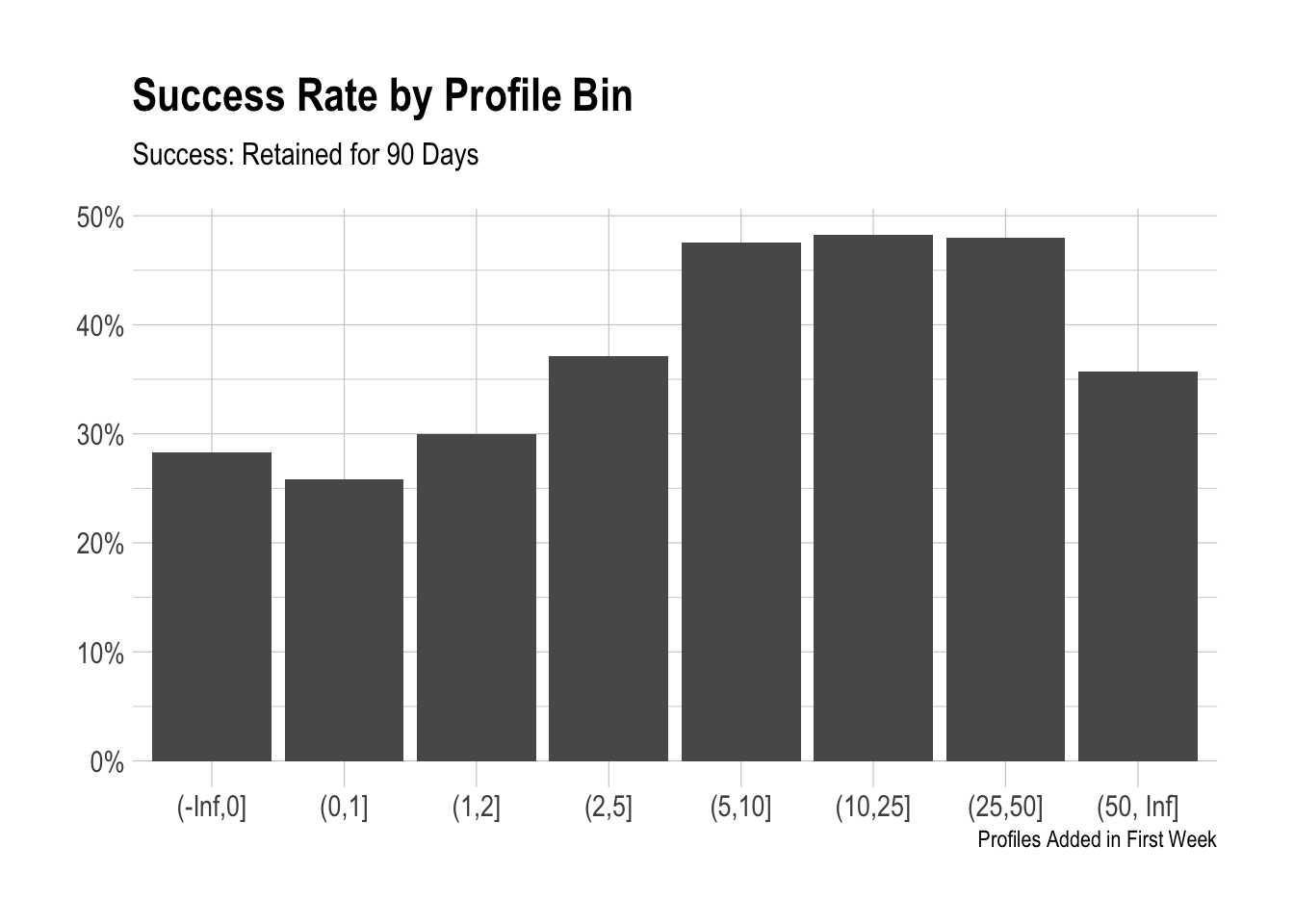
We can see that adding a single profile doesn’t quite lead to success. The biggest jump in the success rate comes between two and ten profiles.

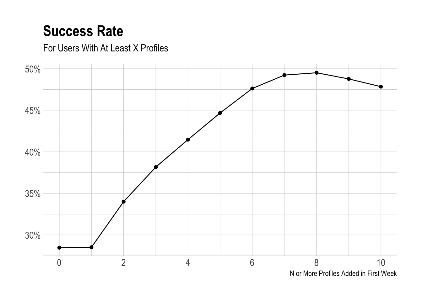
There don’t appear to be any inflection points here, and we can’t really influence how many social accounts users have in general, so I may not recommend using profiles in an activation metric, despite the strong correlation.

Days Active

Finally we’ll look at the number of days active in the first week. How are there successful users with no days active? These users didn’t send any updates. We’ll have to look into that.

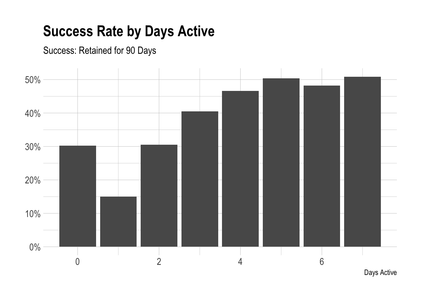
We see a significant jump in the success rate when the number of days active increases from one to two. Therefore, I might suggest an activation metric of at least 3 updates, at least 2 profiles, and at least 2 days active in the first week.

Activation Metric

Let’s see how many users activated, if we use this metric, and what their retention rate was.

# determine if activated
users <- users %>% 
  mutate(activated = (updates >= 3 & days_active >= 2)) 

Let’s see the proportion of users that activated.

# get activation rate
users %>% 
  group_by(activated) %>% 
  summarise(users = n_distinct(user_id)) %>% 
  mutate(percent = users / sum(users))

## # A tibble: 2 x 3
##   activated   users percent
##   <lgl>       <int>   <dbl>
## 1 F         1184805   0.827
## 2 T          247443   0.173

Around 17% of users activated. Let’s see how likely activated users are to be retained compoared to unactivated users.

# see success rate
users %>% 
  group_by(activated, successful) %>% 
  summarise(users = n_distinct(user_id)) %>% 
  mutate(percent = users / sum(users)) %>% 
  filter(successful)

## # A tibble: 2 x 4
## # Groups:   activated [2]
##   activated successful  users percent
##   <lgl>     <lgl>       <int>   <dbl>
## 1 F         T          307285   0.259
## 2 T         T          100365   0.406

Around 26% of users that did not activate were retained for three months, whereas 41% of users that activated were retained. Activated users are more than 60% more likely to be retained for three months by this definition.