Equal Pay Report 2018

Data Collection

The data we’ll use in this analysis comes from this spreadsheet. We’ll simply read in a CSV downloaded from this sheet.

# read csv
salaries <- read.csv("~/Downloads/salaries.csv", header = TRUE)

Now we’re ready for some exploratory analysis.

Global Summary Statistics

Let’s begin by describing the distribution of salaries for all team members of Buffer. It might be helpful to define a couple fields in our dataset. The salary field contains the totol pre-tax salaries of team members before tax in US dollars. This includes dependent grants and the choice to receive a higher salary instead of stock options.

The base_salary field contains the base salary as calculated by our new salary formula. This excludes dependent grants and salary choices.

In this analysis I chose to focus on the salary values, because that is what people take home (for the most part).

# summarise salary
summary(salaries$salary)

##    Min. 1st Qu.  Median    Mean 3rd Qu.    Max. 
##   69483   86864  109350  114211  128412  265315

The median salary at Buffer is $109K and the average is $114K. We can plot the distribution of salaries across Buffer.

# define cuts
cuts <- seq(60000, 280000, 20000)

# define salary buckets
salaries <- salaries %>% 
  mutate(salary_bin = cut(salary, breaks = cuts, dig.lab = 10))

# plot distribution of salaries
salaries %>% 
  count(salary_bin) %>% 
  ggplot(aes(x = salary_bin, y = n)) +
  geom_bar(stat = 'identity') +
  theme_ipsum() +
  theme(axis.text.x = element_text(angle = 45, hjust = 1)) +
  labs(x = NULL, y = "Team Members", title = "Salary Distribution")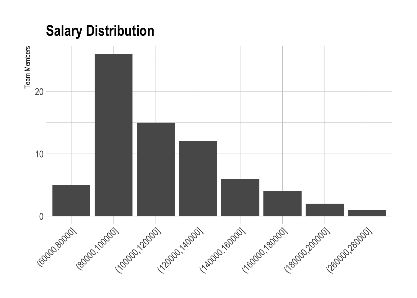

The most common salary “bin” is 80-100K. Let’s break salary down by gender now.

Average Salary by Gender

We can quickly calculate the average and median salaries for both men and women at Buffer.

# calculate average and median salaries
salaries %>% 
  group_by(gender) %>% 
  summarise(average_salary = mean(salary), median_salary = median(salary))

## # A tibble: 2 x 3
##   gender average_salary median_salary
##   <fct>           <dbl>         <dbl>
## 1 female         106819         94546
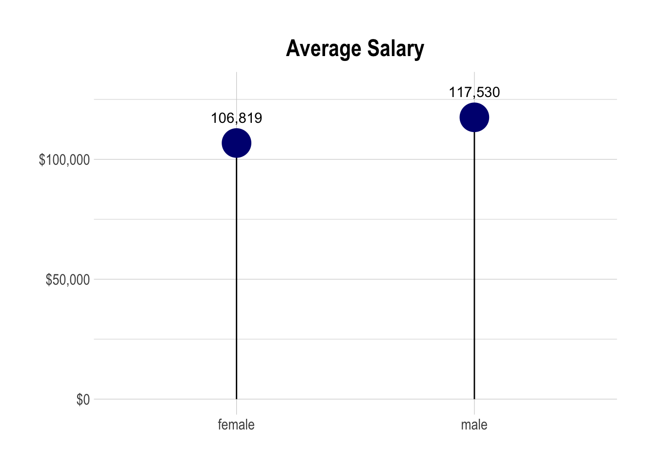
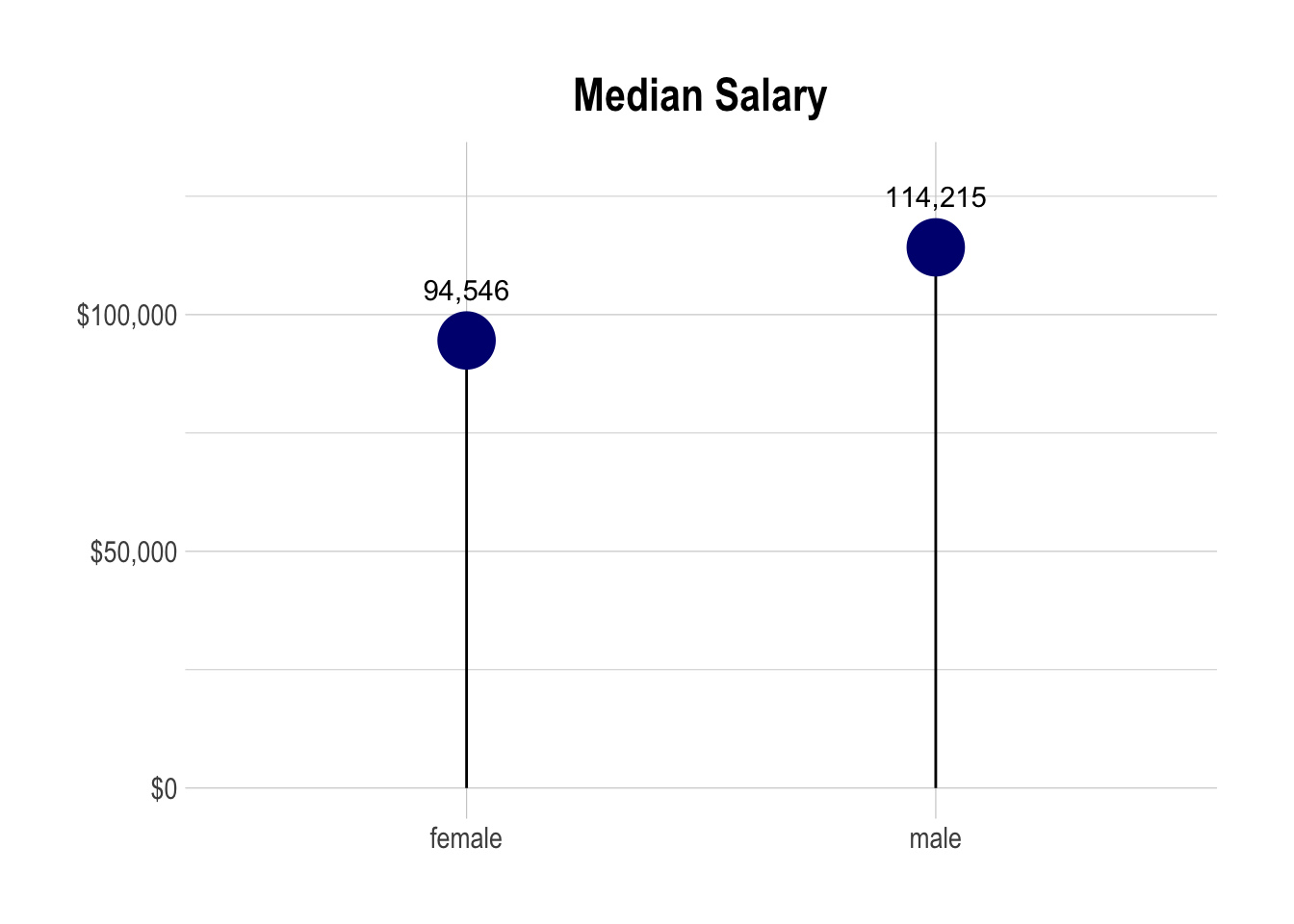
## 2 male           117530        114215

The average salary for females at Buffer is $106,808 and the median is $94,546. The average salary for men is $117,530 and the median is $114,215.

If we look at averages, men earn around 10% more than women – if we look at medians, men earn around 21% more than women!

This discrpency can be surprising, especially for a company with a salary formula! Gender does not enter the salary formula in any way. However, there is something interesting going on - let’s take a closer look at the data.

Technical and Non-Technical Roles

I’m not the biggest fan of this terminology, but it can be useful to describe roles. Technical roles include engineering, data, design, product, and our full-stack marketer. Non-technical roles include marketing, leadership, and advocacy.

If we calculate the average salaries for technical and non-technical roles, we might see something interesting.

# calculate average salaries for tech and non-tech roles
salaries %>% 
  group_by(role_type, gender) %>% 
  summarise(average_salary = mean(salary))

## # A tibble: 4 x 3
## # Groups:   role_type [?]
##   role_type     gender average_salary
##   <fct>         <fct>           <dbl>
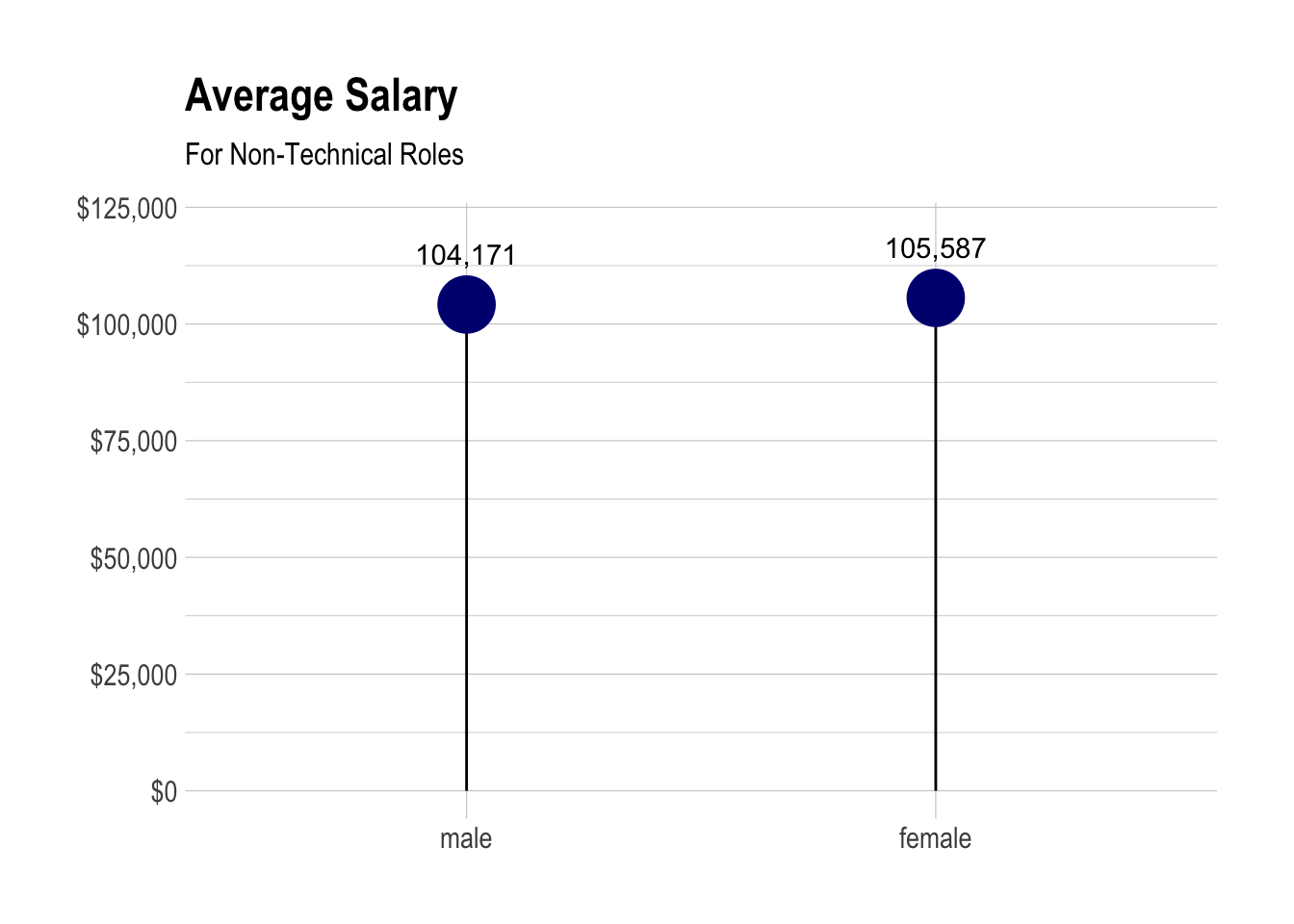
## 1 non-technical female         105587
## 2 non-technical male           104171
## 3 technical     female         112363
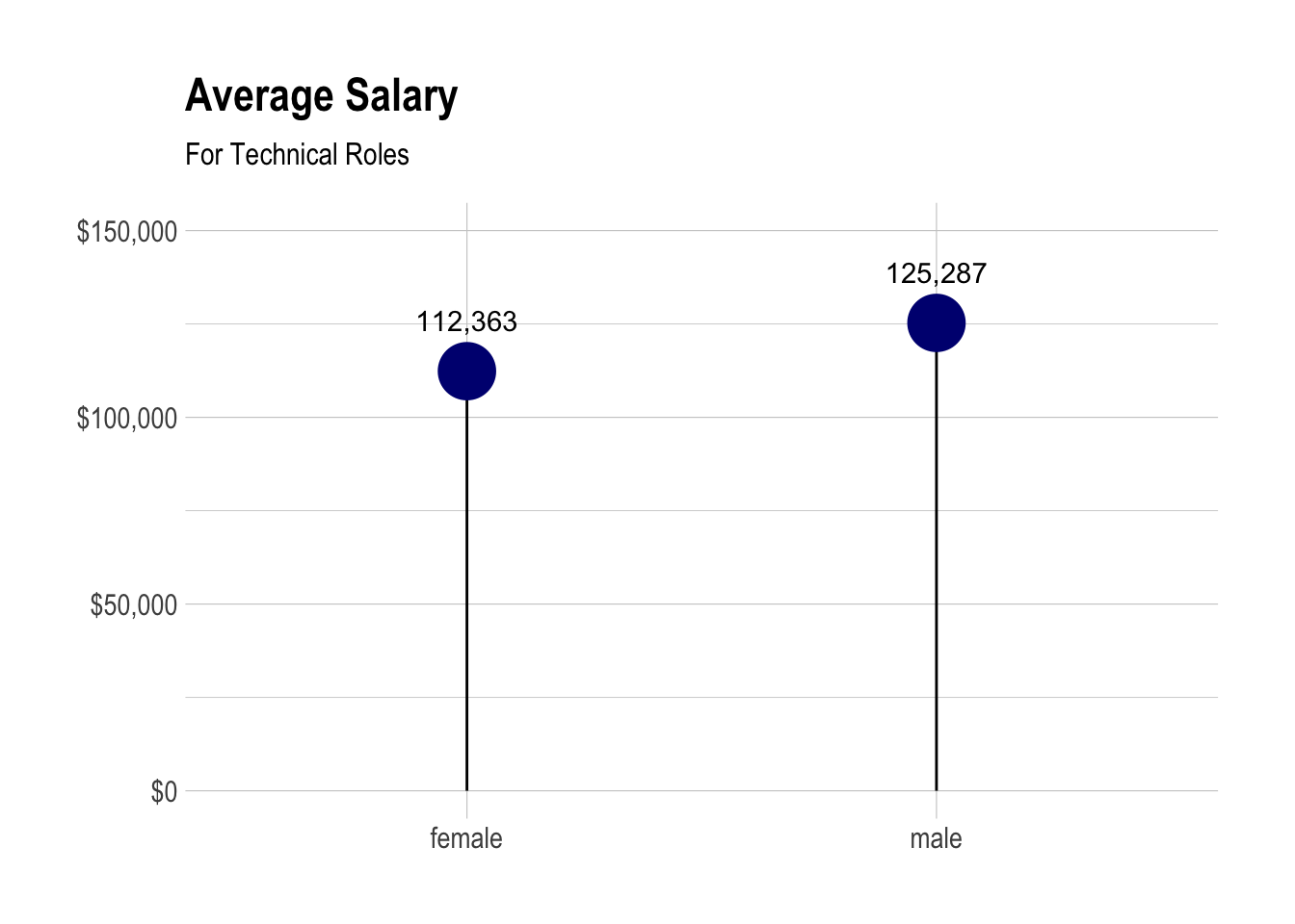
## 4 technical     male           125287

This is interesting. If we segment team members by their role type, we can see that women earn around 1% more than men in non-technical roles, and men earn around only 12% more than women in technical roles.

This seems to explain the overall difference in average salaries. There are more men in technical roles, which tend to demand higher salaries. That, coupled with the fact that men earn more on-average than women in technical roles, leads to the 10% difference in the overall average salary.

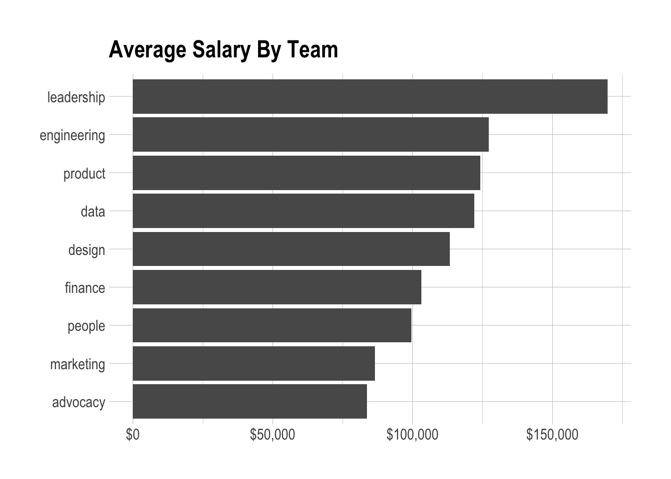
Salaries by Team

We can also plot the average salary for each team at Buffer.

salaries %>%
  group_by(team) %>%
  summarise(average_salary = mean(salary)) %>% 
  arrange(desc(average_salary))

## # A tibble: 9 x 2
##   team        average_salary
##   <fct>                <dbl>
## 1 leadership          169675
## 2 engineering         127177
## 3 product             124146
## 4 data                121996
## 5 design              113257
## 6 finance             103073
## 7 people               99498
## 8 marketing            86506
## 9 advocacy             83751

Interesting stuff overall!