An analysis of #bufferchat tweets

Collecting the tweets

We can use the rtweet package from Michael Kearney to collect the tweets. For this analysis, I connected to Twitter’s streaming API to collect all tweets containing the hashtag “#bufferchat”, but you could also do a basic search to grab the last n tweets containing the term.

To access the API, you’ll need to create an app at apps.twitter.com and obtain your API keys.

# load packages
library(rtweet); library(dplyr); library(lubridate); library(ggplot2)

# create access token
# twitter_token <- create_token(app = "julian_rtweet_app",
#                              consumer_key = Sys.getenv("TWITTER_API_CLIENT_ID"), 
#                              consumer_secret = Sys.getenv("TWITTER_API_CLIENT_SECRET"))

# save token
# saveRDS(twitter_token, "~/.rtweet-oauth.rds")

Now that we’ve created an access token, we can specify the parameters to capture a live stream of tweets from Twitter’s REST API. By default, the stream_tweets function will stream for 30 seconds and return a random sample of tweets. To modify the default settings, stream_tweets accepts several parameters, including q (query used to filter tweets), timeout (duration or time of stream in seconds), and file_name (path name for saving raw json data).

# specify parameters for twitter stream
keywords <- "#bufferchat"
streamtime <- 60 * 70
filename <- "bufferchat.json"

Once the parameters are set, we can initiate the stream.

# stream tweets
tweets_json <- stream_tweets(q = keywords, timeout = streamtime, file_name = filename)

# parse from json file
tweets <- parse_stream(filename)

Awesome, we have 1377 tweets from this week’s Bufferchat. Here is a sample of what the data looks like.

head(tweets %>% select(screen_name:status_id))

##       screen_name    user_id          created_at          status_id
## 1 TheEventsSeeker  724335139 2017-10-25 15:50:46 923215265453633537
## 2     auraeleonor  136499071 2017-10-25 15:50:56 923215306738290688
## 3     MalharBarai   57591036 2017-10-25 15:51:32 923215460035837952
## 4   digitalpratik 3184398348 2017-10-25 15:52:11 923215623106080768
## 5  Haylee_Cornett  202346411 2017-10-25 15:52:29 923215699069276160
## 6       DewiEirig   19086504 2017-10-25 15:52:48 923215778702340096

We can extract data about the users that sent the tweets as well.

# get user data
users <- users_data(tweets)

Now, let’s do some exploratory analysis.

Graphs and things

Once parsed, the ts_plot() function provides a quick visual of the frequency of tweets. By default, ts_plot() will try to aggregate time by the day, but we can aggregate by minute instead.

# plot frequency of tweets
ts_plot(tweets, by = "minutes")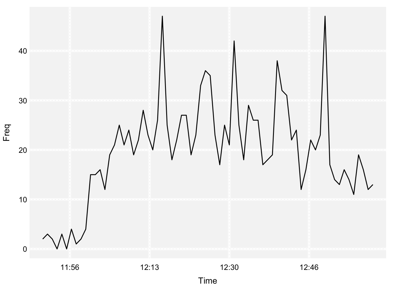

Today’s bufferchat was scheduled to begin at 12:00pm ET and last for one hour. I turned the stream on shortly before 12 and left it on for 70 minutes. We can see that the frequncy of tweets picks up shortly after 12 and starts to decline around 12:40pm.

We can see that there are distinct local peaks in this time series. I have a suspicion that these occur around the time that the Buffer twitter account releases the questions. Let’s try to plot these times on the same plot. To get these times, we’ll filter our tweets to only include tweets from the Buffer account that were not replies (there are lots of replies).

# get buffer tweets
tweets %>%
  filter(screen_name == 'buffer' & is.na(in_reply_to_status_user_id)) %>%
  select(text)

##                                                                                                                                                      text
## 1        Welcome to #bufferchat! (This is the 2nd of 2 chats this week) Anyone joining in the chat for the first time? \U0001f60a https://t.co/6bjHNRtdOY
## 2  Let’s kick off #bufferchat with an icebreaker! Where are you tweeting from & what's one of your favorite teams? \U0001f914 https://t.co/NeBmwfaYTB
## 3             Quick #bufferchat ask: up for including “A1, A2…” in your answer tweets? We’d love to include your insights in our… https://t.co/Tdm3TDLAKe
## 4                                     Q1: How many people are on your particular team? Does your team have a name? :) #bufferchat https://t.co/jbJd41ZLkP
## 5                                       Q2: Who do you work most closely with on your team? How do you work together? #bufferchat https://t.co/BFMRMcDphY
## 6                     Q3: Anyone have great tips for structuring meetings or brainstorms with your team? What works really well?… https://t.co/6VZRr8HMQR
## 7                                           Q4: What are some awesome tools that support team collaboration, and how? #bufferchat https://t.co/IgUaAEXlUJ
## 8                                                 Q5: What’s your advice for working through conflicts within a team? #bufferchat https://t.co/t16hLcffCg
## 9                                  Q6: What are some ideal ways for a team to get to know each other and build trust? #bufferchat https://t.co/U3u0yBKNc9
## 10                                                 Q7: Do you have any awesome team collaboration successes to share? #bufferchat https://t.co/RQaCNeY7sO
## 11                                                     Bonus! How would you summarize today’s #bufferchat learnings in one tweet? https://t.co/dsGeb2Xwdr
## 12             Thank you all so much for your awesome insights! Look for our #bufferchat recap here soon: https://t.co/a3JgZpWTMa https://t.co/H0nN0TXJjD

That’s them! Let’s grab the times of these tweets.

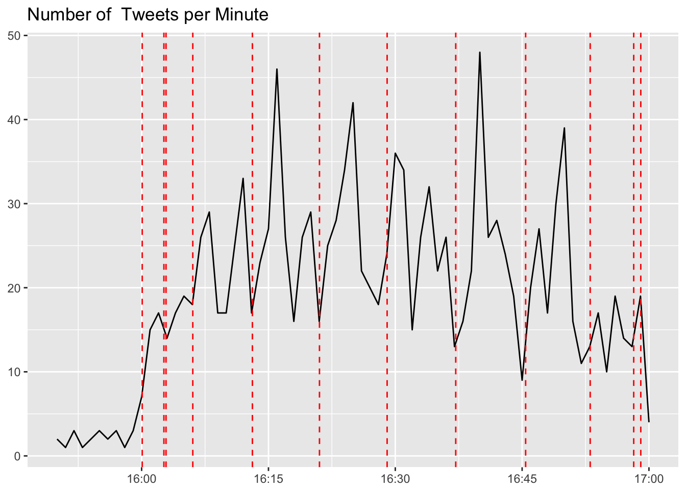
The red dashed lines represent the times in which the Buffer account tweeted a question or announcement. We can see that in the minutes following a tweet, there tended to be an increase in activity.

Sentiment analysis

The Buffer team is the happiest group of people I’ve been around, and it shows in our communication. I would guess that the bufferchat tweets have very high sentiment scores – let’s check and see.

# we'll use the tidytext package
library(tidytext); library(tidyr)

# unnest tokens
words <- tweets %>%
  unnest_tokens(word, text) %>%
  anti_join(stop_words, by = 'word')

As discussed above, there are a variety of methods and dictionaries that exist for evaluating the opinion or emotion in text. The tidytext package contains several sentiment lexicons in the sentiments dataset.

sentiments

## # A tibble: 23,165 x 4
##           word sentiment lexicon score
##          <chr>     <chr>   <chr> <int>
##  1      abacus     trust     nrc    NA
##  2     abandon      fear     nrc    NA
##  3     abandon  negative     nrc    NA
##  4     abandon   sadness     nrc    NA
##  5   abandoned     anger     nrc    NA
##  6   abandoned      fear     nrc    NA
##  7   abandoned  negative     nrc    NA
##  8   abandoned   sadness     nrc    NA
##  9 abandonment     anger     nrc    NA
## 10 abandonment      fear     nrc    NA
## # ... with 23,155 more rows

The three general-purpose lexicons are:

• AFINN from Finn Årup Nielsen
• bing from Bing Liu and collaborators
• nrc from Saif Mohammad and Peter Turney

We’ll use the bing lexicon to plot the sentiment of the tweets during today’s chat.

sentiment <- words %>%
  mutate(created_at_minute = floor_date(created_at, unit = "minutes")) %>%
  inner_join(get_sentiments("bing"), by = 'word') %>%
  count(created_at_minute, sentiment) %>%
  spread(sentiment, n, fill = 0) %>%
  mutate(sentiment = positive - negative)

Now we can plot these sentiment scores across the entirety of the chat.

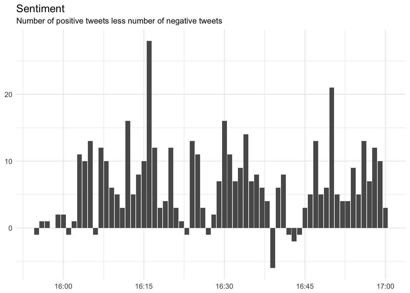
I refuse to believe that there are minutes in which there are more negative tweets than positive, so let’s take a look at some of these so-called “negative” tweets.

@buffer I’ve seen #bufferchat before but always seem to miss them. This is my first.

This isn’t negative, but I see why our approach might classify it as negative.

@SamanthaS_PR @buffer Hello! This is only my third #bufferchat but I am a bit addicted… be warned

This one also isn’t negative, but does include a couple of words that could be described as negative. It’s more playful than anything.

Missed the Periscope. It wouldn’t load…

Fine. Maybe there is one negative tweet. You get the idea!

Mapping the tweets

I’ve always thought that it fun to map where the tweets come from. In the end, we’ll be able to create a map like this one.

We’ll need to use the location field in the users data frame that we created earlier. In order to get the coordinates for these locations, we’ll use Google Maps’ geocoding API. It is very helpful to go there and get an API key.

The code below sets up a funcion we can call to call the API for each location in the users dataset.

library(RCurl)
library(RJSONIO)
library(plyr)

# build URL to access api
url <- function(address, return.call = "json", sensor = "false") {
  
  key <- Sys.getenv('GEOCODE_API_KEY')
  
  root <- "https://maps.google.com/maps/api/geocode/"
  u <- paste(root, return.call, "?address=", address, "&key=", key, "&sensor=", sensor, sep = "")
  
  return(URLencode(u))
}

# function to parse the results:
geoCode <- function(address, verbose = FALSE) {
  
  if(verbose) cat(address, "\n")
  u <- url(address)
  doc <- getURL(u)
  x <- fromJSON(doc,simplify = FALSE)
  print(x$status)
  
  if(x$status == "OK") {
    
    lat <- x$results[[1]]$geometry$location$lat
    lng <- x$results[[1]]$geometry$location$lng
    location_type  <- x$results[[1]]$geometry$location_type
    formatted_address  <- x$results[[1]]$formatted_address
    
    return(c(lat, lng, location_type, formatted_address))
    Sys.sleep(0.5)
    
  } else {
    
    return(c(NA,NA,NA, NA))
    
  }
}

# function to get coordinates
get_coordinates <- function(locations) {
  
  # apply geCode function to all locations
  coordinates  <- ldply(locations, function(x) geoCode(x))
  
  # rename columns
  names(coordinates)  <- c("lat","lon","location_type", "formatted")
  
  # set latitude and longitude as numeric
  coordinates$lat <- as.numeric(coordinates$lat)
  coordinates$lon <- as.numeric(coordinates$lon)
  
  # return dataframe
  return(coordinates)
}

To get the coordinates for these bufferchat users, we can use the following two commands.

# get locations of users
locations <- users[!is.na(users$location),]$location

# geocode vector with addresses
coordinates <- get_coordinates(locations)

Now we can build the map.

# get world map
library(ggalt); library(ggthemes)

# get world map
world <- map_data("world")
world <- world[world$region != "Antarctica",]

# plot tweets on a world map
ggplot() + 
  geom_map(data = world, map = world, aes(x = long, y = lat, map_id = region), 
           color="white", fill="#7f7f7f", size=0.05, alpha=1/4) +
  geom_point(data = coordinates, aes(x = lon, y = lat), alpha = 0.3, size = 2, position = 'jitter') +
  scale_color_tableau() +
  coord_proj("+proj=wintri") +
  theme(strip.background=element_blank()) +
  theme_map() 

That’s it for now! What do you all think? Anything else you’d like to see?