Towards the end of 2017, Buffer sent out a survey to gauge the state of social media going into 2018. We had over 1700 responses, which we downloaded as a csv file and stored as an R data object. The questions and responses can be viewed here.
The survey consisted of 30 questions about how users use social media.
# get response data
responses <- readRDS('state-of-social.rds')
The data is quite messy and untidy. Let’s begin by addressing the column names. We can use the safe_names() function in the buffer package to take care of uppercase letters and periods in the column names.
# clean up column names
colnames(responses) <- safe_names(colnames(responses))
The column names in the dataframe are just the questions. These are too long to work with efficiently, so we’ll replace them with question numbers q1 through q87. You might wonder why there are 88 columns in our dataframe. We have so many columns because some of the questions in the survey allow for multiple responses.
For example, the question “Which of the following channels does your business use currently?” could be answered with any combination of social networks, e.g. Facebook, Facebook and Snapchat, Linkedin and Twitter and Facebook, etc. This survey question can be broken apart into eight individual questions corresponding to each social network. The question really asks “does your business use Facebook?”, “does your business use Twitter?”, “does your business use Pinterest?”, etc.
Now, let’s create a lookup table that will help us reference the worded question for each question number.
# create lookup table for questions
questions <- data_frame(number = character(87), question = character(87))

# set the question numbers
questions$number <- paste0('q', seq(1:87))

# set the worded questions
questions$question <- colnames(select(responses, -x_))
Nice, now we’ll be able to look up the question for each question number. Let’s replace the column names in our responses dataframe.
# set column names
column_names <- c('user_id', questions$number)

# replace column names
colnames(responses) <- column_names
Alright, I think we’re ready for some exploratory analysis!
Exploratory analysis
The first few questions we ask are about the companies the respondents work for. We ask about their industries, size, and social media profiles. Let’s plot a few histograms to see what some common combinations are.
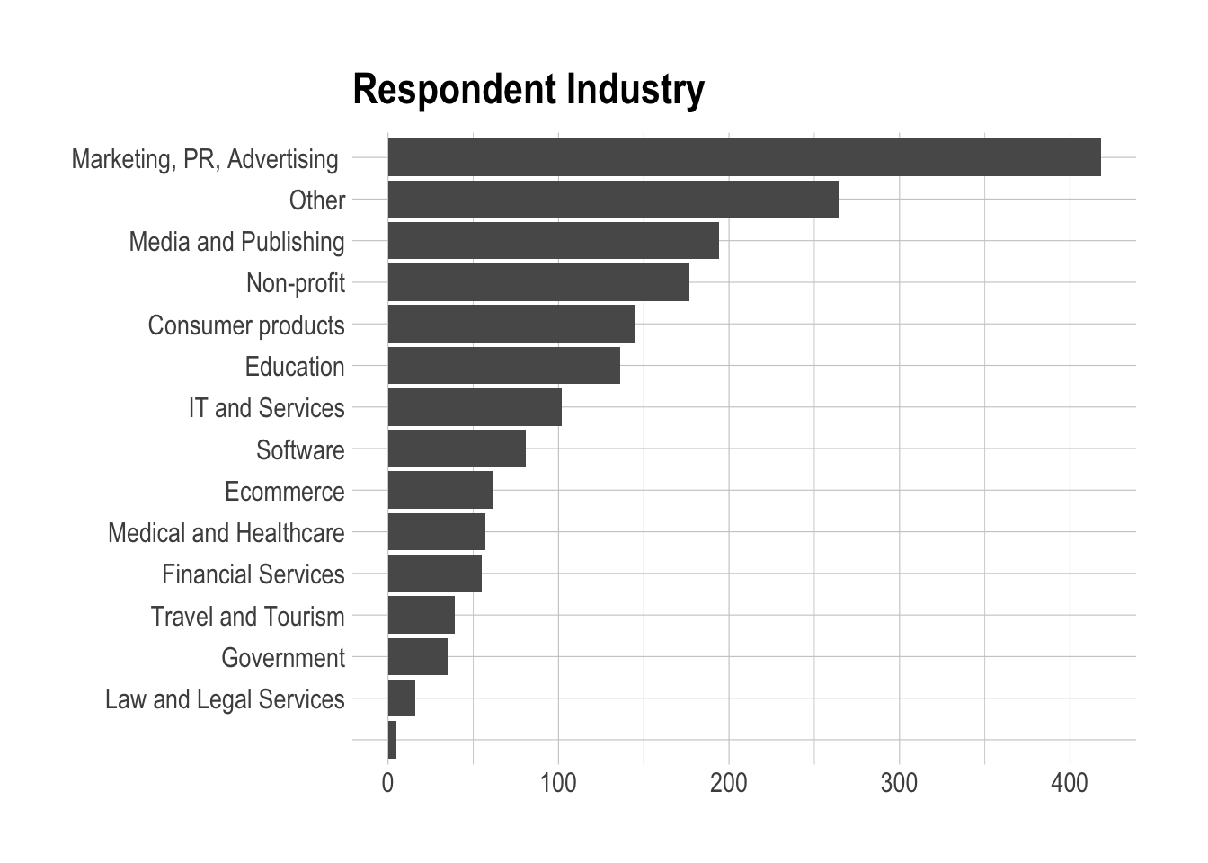
We can see that over 400 respondents work in marketing, PR, or advertising. They represent around 23% of all respondents. Media and publishing, non-profits, consumer products, and education make up another 37% of respodents.
Let’s take a look at the sizes of these commpanies.
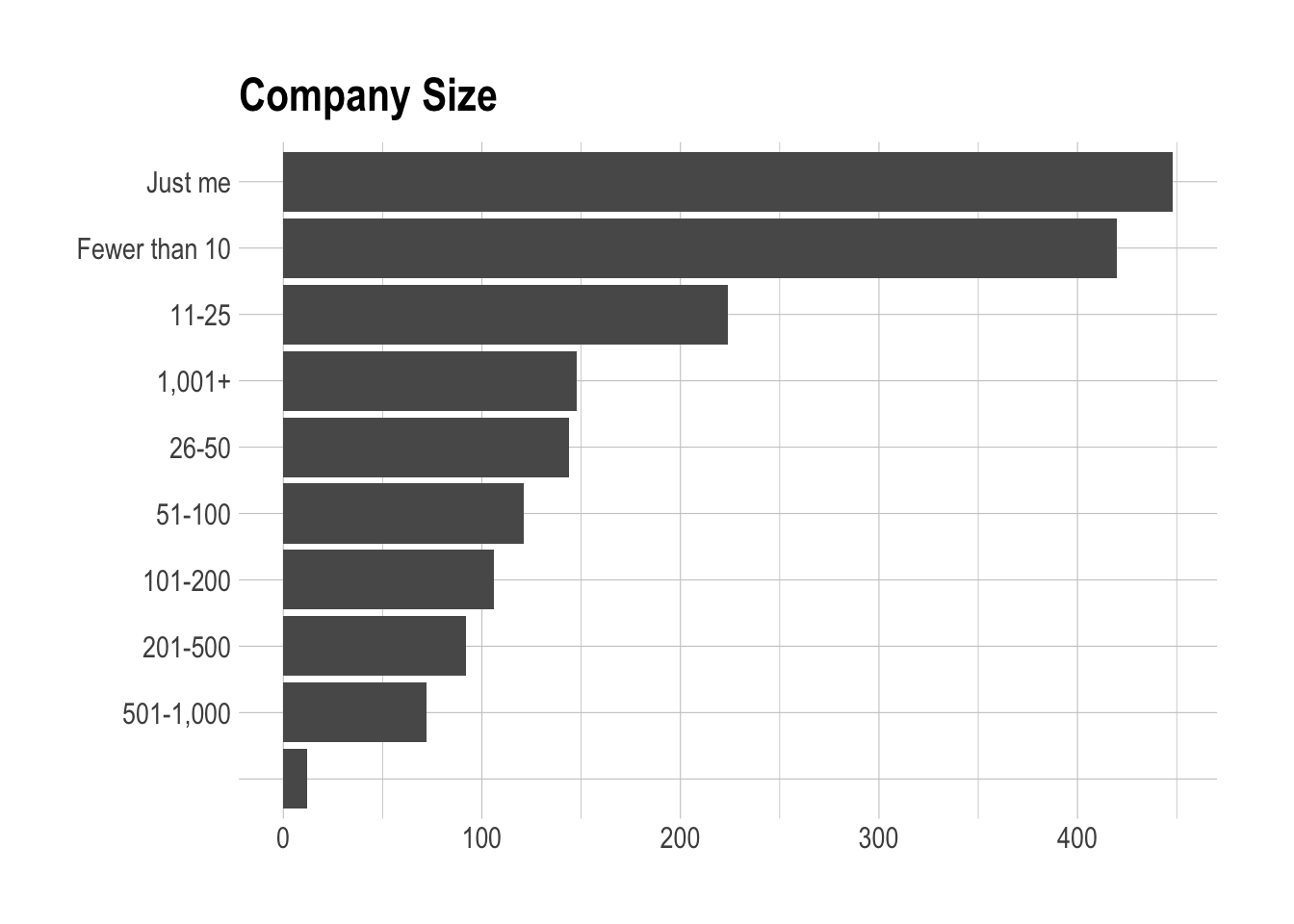
Most of the respondents worked for small companies. The most common response company size was just a single person! Let’s explore the relationship between the two.
table(responses$q1, responses$q2)##
## 1,001+ 101-200 11-25 201-500 26-50
## 4 0 0 0 0 0
## Consumer products 1 19 7 14 9 10
## Ecommerce 0 2 4 8 2 6
## Education 2 23 11 7 19 4
## Financial Services 0 13 5 8 3 8
## Government 0 12 7 6 5 1
## IT and Services 0 12 3 17 7 8
## Law and Legal Services 0 3 0 4 0 2
## Marketing, PR, Advertising 0 8 9 59 8 29
## Media and Publishing 1 9 7 18 4 12
## Medical and Healthcare 0 13 2 7 4 5
## Non-profit 1 6 17 32 7 26
## Other 2 20 22 30 12 18
## Software 1 5 8 13 7 12
## Travel and Tourism 0 3 4 1 5 3
##
## 501-1,000 51-100 Fewer than 10 Just me
## 0 0 0 1
## Consumer products 10 11 35 29
## Ecommerce 2 5 15 18
## Education 9 12 28 21
## Financial Services 1 5 5 7
## Government 3 0 0 1
## IT and Services 9 6 25 15
## Law and Legal Services 2 2 2 1
## Marketing, PR, Advertising 5 16 130 154
## Media and Publishing 7 10 46 80
## Medical and Healthcare 2 7 8 9
## Non-profit 5 18 41 24
## Other 11 17 54 79
## Software 4 11 17 3
## Travel and Tourism 2 1 14 6We can see that the most common responses are Marketing, PR, and Advertising companies with fewer than 10 employees, including single employees.
We can plot the combinations with at least 25 respondents.
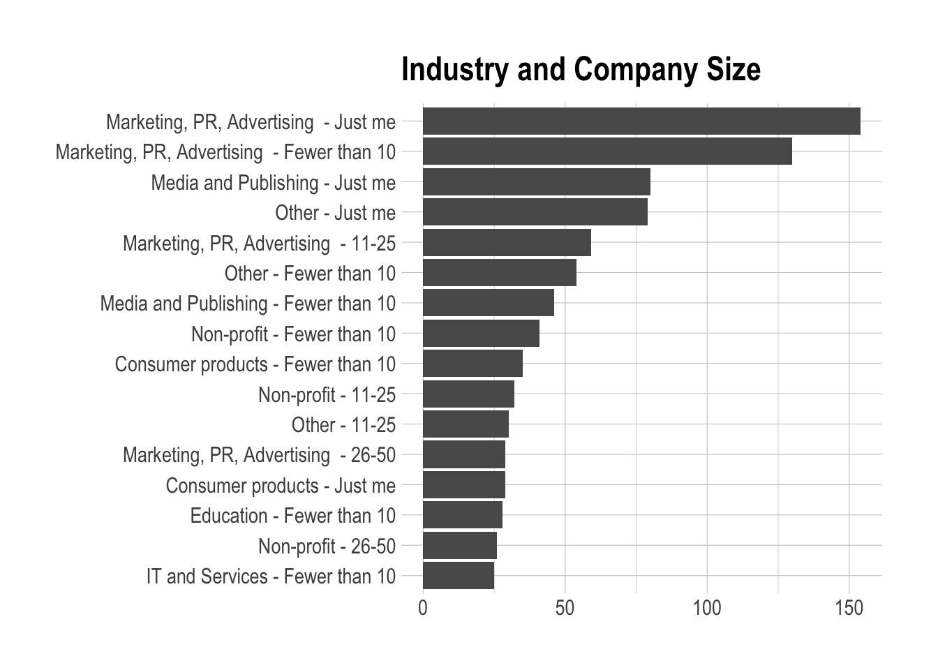
We can see that only a few of the most popular combinations have a team size over 10. Now let’s try to answer a few specific questions.
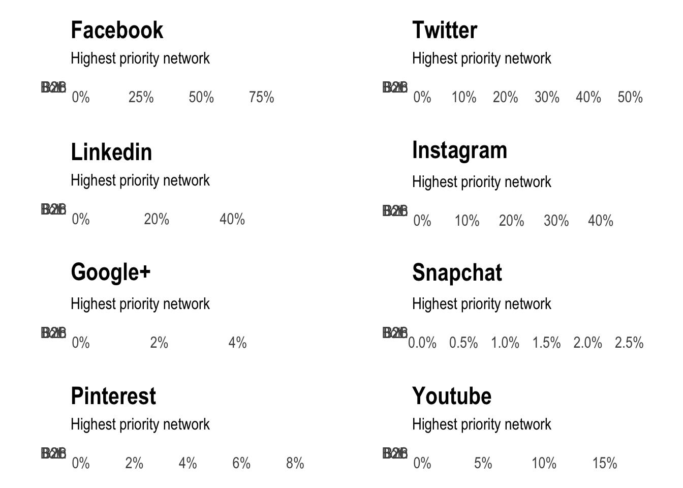
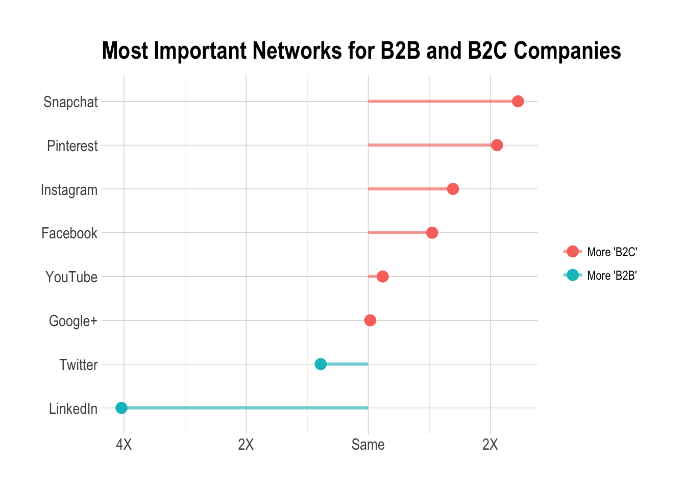
Which social media network is the highest priority for B2C and B2B businesses?
In question four, we asked whether the respondents’ companies were business-to-business (B2B) or business-to-consumer (B2C). Questions 14 through 21 correspond to the responses of the question “Which of the following channels are the highest priority for your business?”
We can try to determine if there are any significant differences in priorities for B2B and B2C companies. We treat the answers to questions 14 through 21 as individual responses, even though they are in fact responses to a single question (question number 7 in the original Typeform survey).
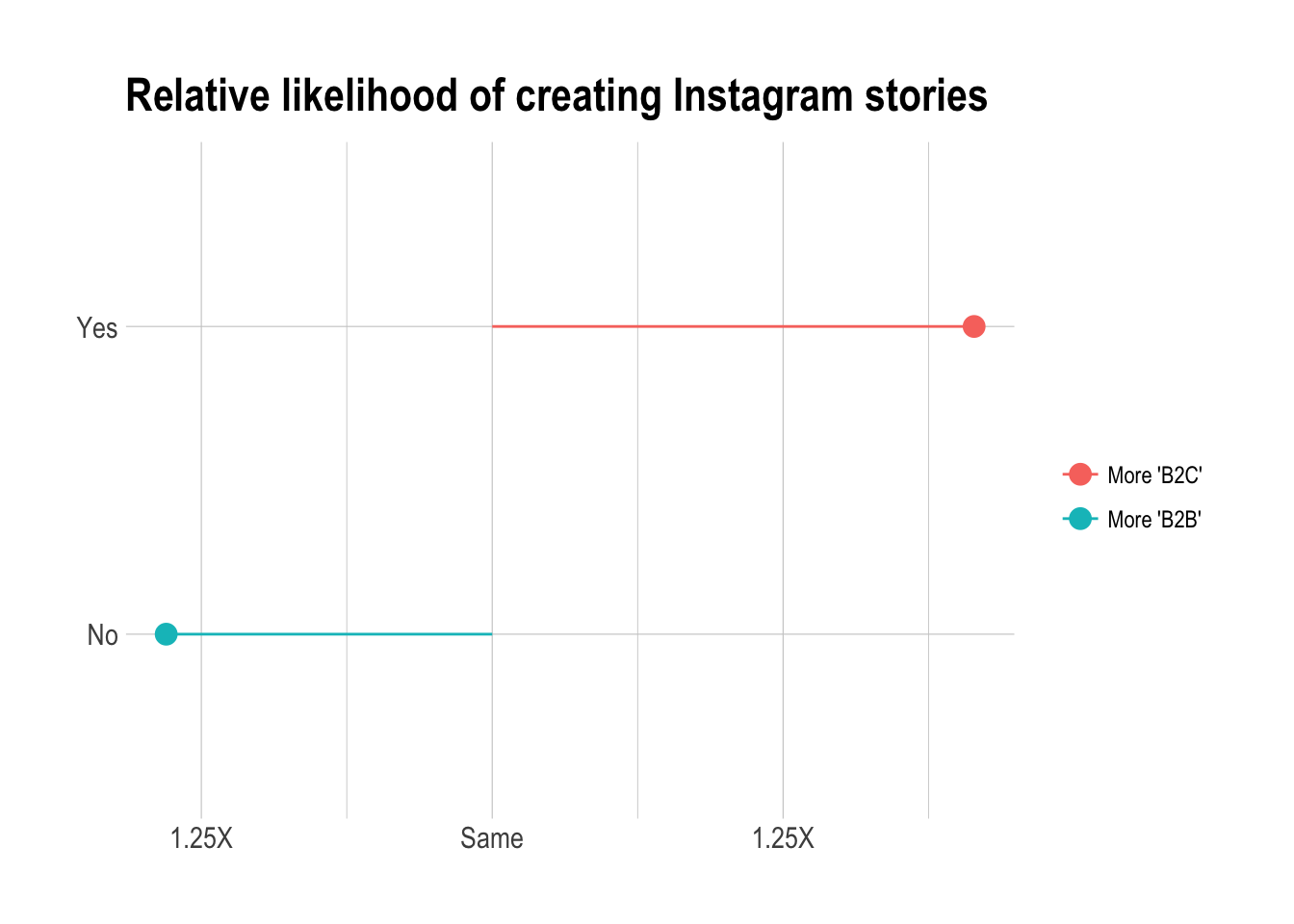
Are B2B companies more likely to create Instagram strategy?
responses %>%
  select(q4, q23) %>%
  group_by(q4, q23) %>%
  summarise(respondents = n()) %>%
  mutate(percent = respondents / sum(respondents)) %>%
  filter(q4 != '' & q23 != '' & q23 == "Yes") %>%
  ungroup() %>%
  mutate(q4 = reorder(q4, percent)) %>%
  ggplot(aes(x = q4, y = percent)) +
  geom_bar(stat = 'identity') +
  scale_y_continuous(labels = percent) +
  coord_flip() +
  theme_ipsum() +
  labs(x = NULL, y = NULL, title = "Instagram strategy",
       subtitle = "Percentage of companies that created a story in 2017")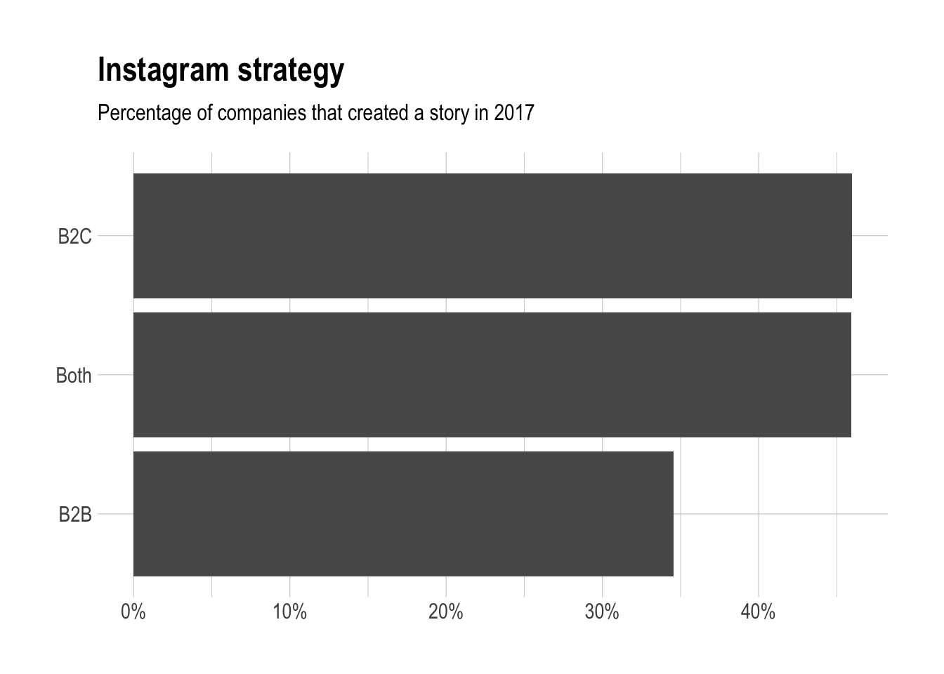
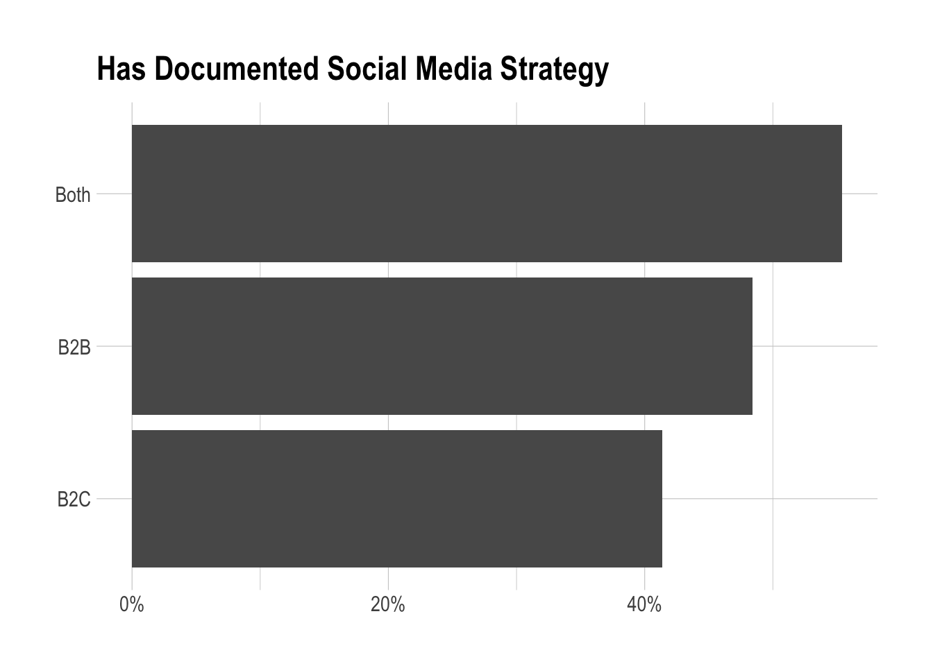
Likelihood of having documented social media strategy
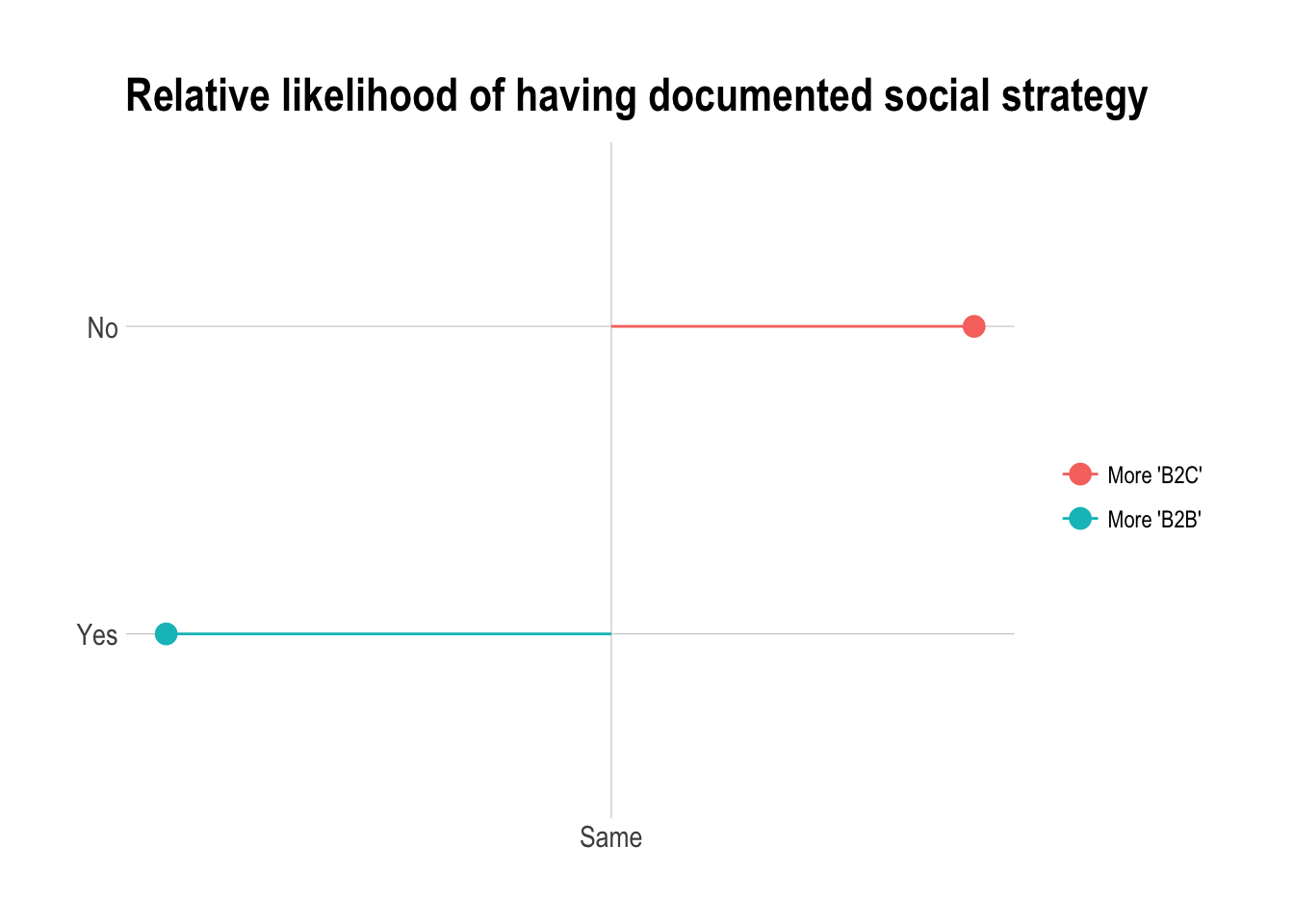
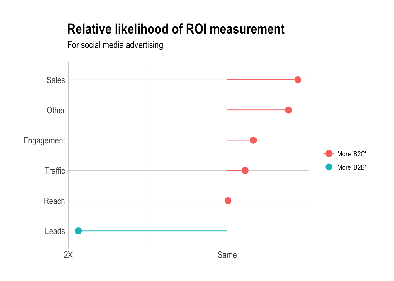
How do B2B and B2C companies measure ROI?
Let’s begin by making a side-by-side plot to show the absolute percentages. We need to do a small transformation first.
# create ROI dataframe
roi <- responses %>%
  select(q4, q74) %>%
  rename(roi = q74) %>%
  filter((q4 == 'B2B' | q4 == 'B2C') & roi != '') %>%
  mutate(roi = as.character(roi))

# replace long engagement value with trucated one
engagement_rows <- grep("Engagement", roi$roi)
roi[engagement_rows, ]$roi <- "Engagement"
Now for the side by side plots.
library(gridExtra)

# b2c plot
b2c <- roi %>%
  filter(roi != '' & q4 == 'B2C') %>%
  group_by(roi) %>%
  summarise(n = n()) %>%
  mutate(percent = n / sum(n)) %>%
  mutate(roi = reorder(roi, n)) %>%
  ggplot(aes(x = roi, y = percent)) +
  geom_bar(stat = 'identity') +
  scale_y_continuous(labels = percent) +
  coord_flip() +
  theme_ipsum() +
  labs(x = NULL, y = NULL, title = "How Social Media ROI is Measured",
       subtitle = "For B2C Companies")

# b2b plot
b2b <- roi %>%
  filter(roi != '' & q4 == 'B2B') %>%
  group_by(roi) %>%
  summarise(n = n()) %>%
  mutate(percent = n / sum(n)) %>%
  mutate(roi = reorder(roi, n)) %>%
  ggplot(aes(x = roi, y = percent)) +
  geom_bar(stat = 'identity') +
  scale_y_continuous(labels = percent) +
  coord_flip() +
  theme_ipsum() +
  labs(x = NULL, y = NULL, title = "",
       subtitle = "For B2B Companies")

# plot two plots together
grid.arrange(b2c, b2b, nrow = 1)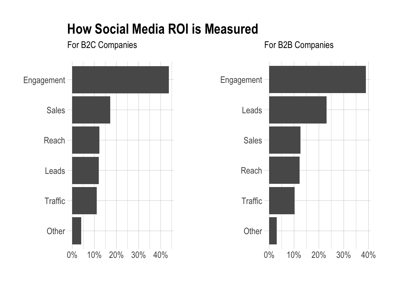
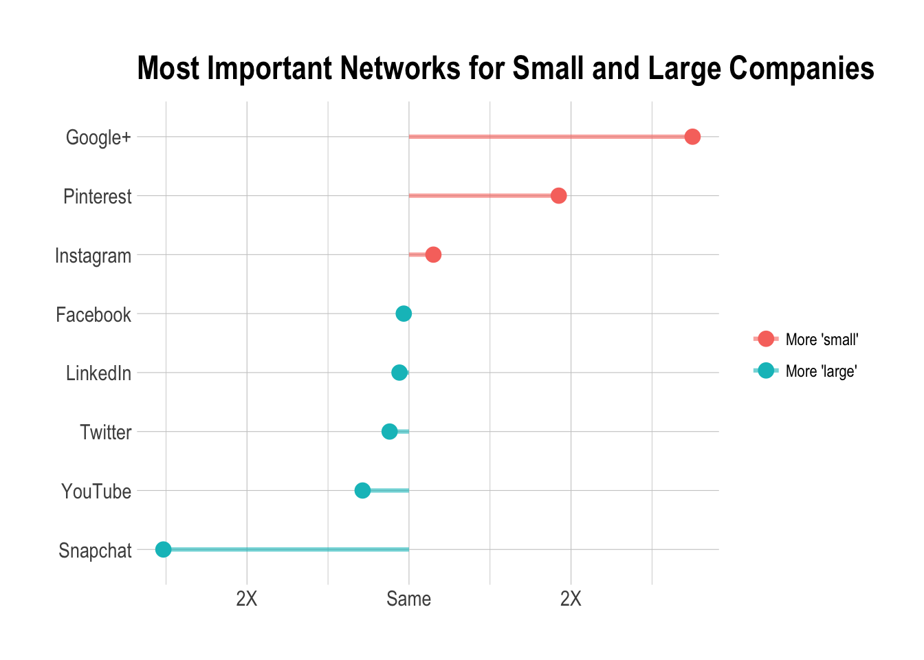
Company size and most important networks
We’ll first determine if a company is considered small or large.
# categorize company size
responses <- responses %>%
  mutate(size = ifelse(q2 == "", NA,
                ifelse(q2 == "Just me", "small",
                ifelse(q2 == "Fewer than 10", "small",
                ifelse(q2 == "11-25", "small",
                ifelse(q2 == "26-50", "small", "large"))))))

table(responses$size)
##
## large small
## 539 1236Now let’s repeat what we’ve done above.

Do large businesses publish videos more frequently?
To answer this question, we’ll need to determine if a business is small or large. We’ll define a small business as one that has between one and fifty employees. We’ll categorize any businesses with over 50 employees as a large business.
# categorize company size
responses <- responses %>%
  mutate(size = ifelse(q2 == "", NA,
                ifelse(q2 == "Just me", "small",
                ifelse(q2 == "Fewer than 10", "small",
                ifelse(q2 == "11-25", "small",
                ifelse(q2 == "26-50", "small", "large"))))))

table(responses$size)
##
## large small
## 539 1236The question regarding video posting frequency is question number 25 in our dataframe. Let’s review the distribution of responses for both small and large businesses.
library(gridExtra)

# small business plot
small <- responses %>%
  filter(q25 != '' & size == 'small') %>%
  group_by(q25) %>%
  summarise(n = n_distinct(user_id)) %>%
  mutate(percent = n / sum(n)) %>%
  mutate(q25 = reorder(q25, n)) %>%
  ggplot(aes(x = q25, y = percent)) +
  geom_bar(stat = 'identity') +
  scale_y_continuous(labels = percent) +
  coord_flip() +
  theme_ipsum() +
  labs(x = NULL, y = NULL, title = "Frequency of Video Uploads",
       subtitle = "For Small Businesses (1-50 employees)")

# large business plot
large <- responses %>%
  filter(q25 != '' & size == 'large') %>%
  group_by(q25) %>%
  summarise(n = n_distinct(user_id)) %>%
  mutate(percent = n / sum(n)) %>%
  mutate(q25 = reorder(q25, n)) %>%
  ggplot(aes(x = q25, y = percent)) +
  geom_bar(stat = 'identity') +
  scale_y_continuous(labels = percent) +
  coord_flip() +
  theme_ipsum() +
  labs(x = NULL, y = NULL, title = "Frequency of Video Uploads",
       subtitle = "For Large Businesses (50+ employees)")

# plot two plots together
grid.arrange(small, large, nrow = 1)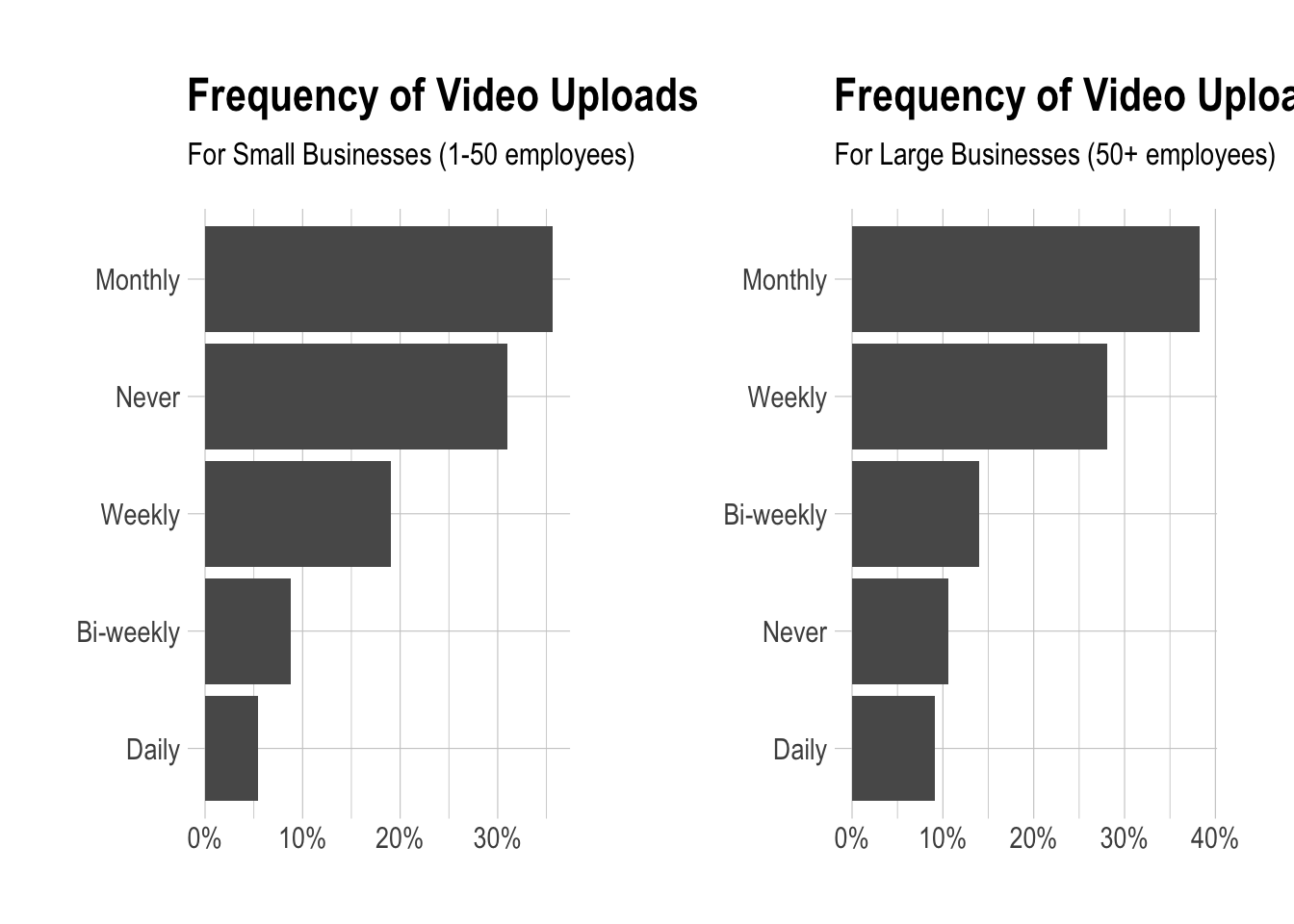
Now we can calculate log ratios to determine if large businesses are more or less likely to publish videos at any frequency.
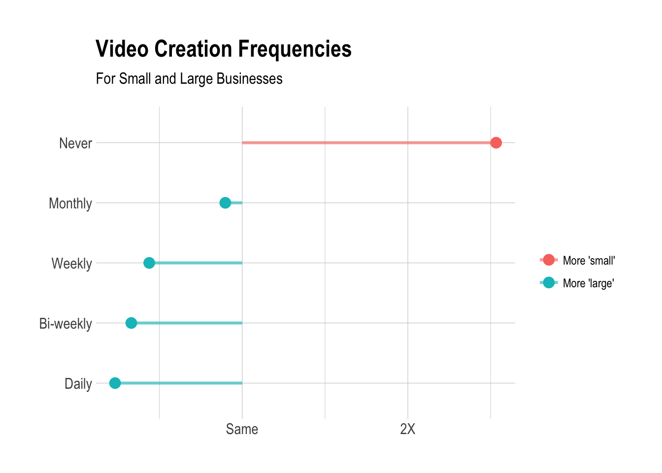
So, it looks like “small” businesses that responded to our survey were more than twice as likely to never create video content than “large” businesses that responded.
Are large companies more likely to have a documented social media strategy?
Let’s take the same approach here, except group on question 5 instead of question 25.
# small business plot
small <- responses %>%
  filter(q5 != '' & size == 'small') %>%
  group_by(q5) %>%
  summarise(n = n_distinct(user_id)) %>%
  mutate(percent = n / sum(n)) %>%
  mutate(q5 = reorder(q5, n)) %>%
  ggplot(aes(x = q5, y = percent)) +
  geom_bar(stat = 'identity') +
  scale_y_continuous(labels = percent) +
  coord_flip() +
  theme_ipsum() +
  labs(x = NULL, y = NULL, title = "Has Documented Social Media Strategy",
       subtitle = "Small Businesses (1-50 employees)")

# large business plot
large <- responses %>%
  filter(q5 != '' & size == 'large') %>%
  group_by(q5) %>%
  summarise(n = n_distinct(user_id)) %>%
  mutate(percent = n / sum(n)) %>%
  mutate(q5 = reorder(q5, n)) %>%
  ggplot(aes(x = q5, y = percent)) +
  geom_bar(stat = 'identity') +
  scale_y_continuous(labels = percent) +
  coord_flip() +
  theme_ipsum() +
  labs(x = NULL, y = NULL, title = "",
       subtitle = "Large Businesses (50+ employees)")

# plot two plots together
grid.arrange(small, large, nrow = 1)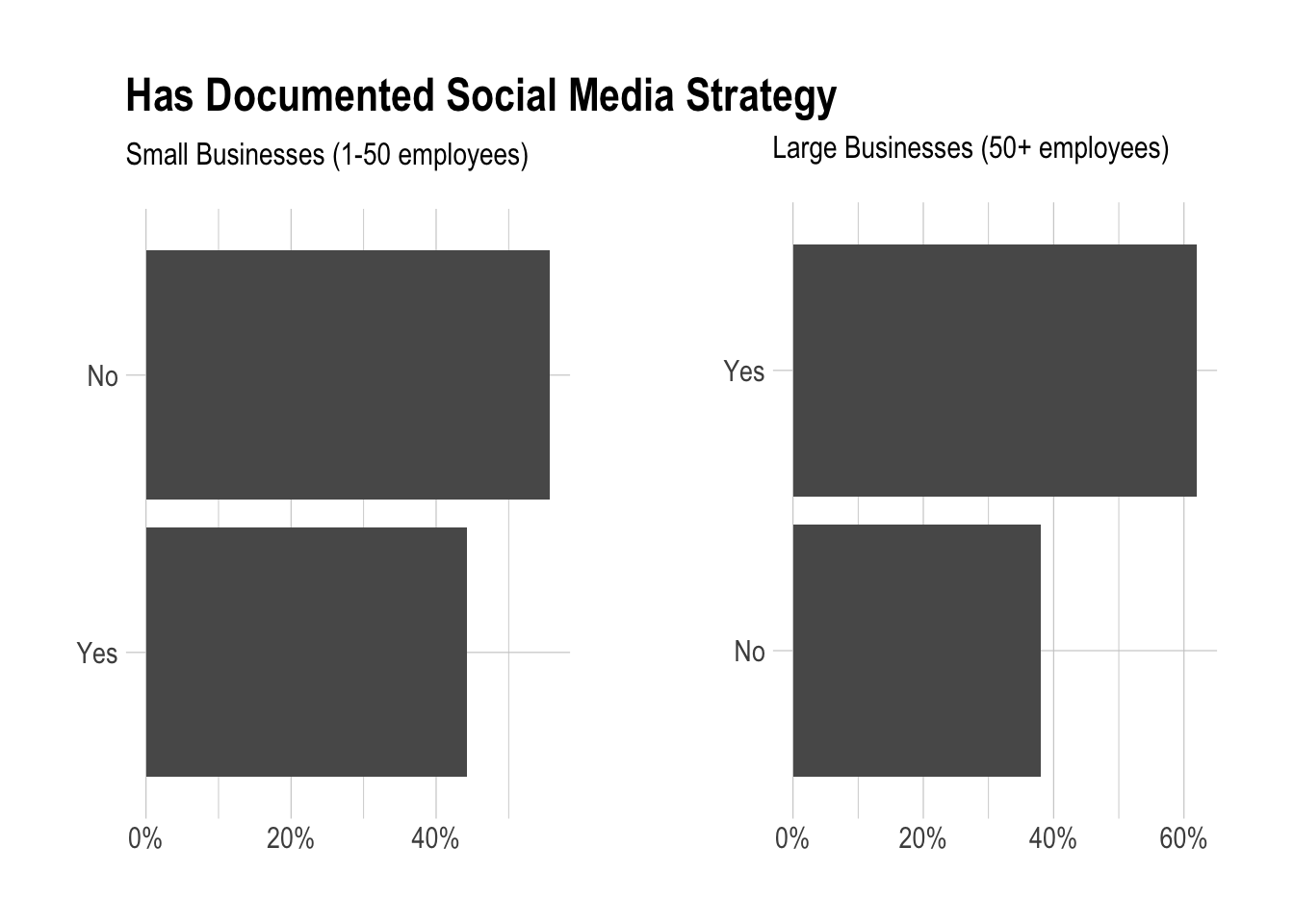
Now let’s plot the log ratios.
# calculate log ratios for the network counts
counts <- responses %>%
  filter(q5 != '') %>%
  count(size, q5) %>%
  spread(size, n, fill = 0) %>%
  mutate(total = small + large,
         small = (small) / sum(small + 1),
         large = (large + 1) / sum(large + 1),
         log_ratio = log2(small / large),
         abs_ratio = abs(log_ratio)) %>%
  arrange(desc(log_ratio))

# plot the ratios
counts %>%
    group_by(direction = ifelse(log_ratio < 0, 'More "small"', "More 'large'")) %>%
    top_n(15, abs_ratio) %>%
    ungroup() %>%
    mutate(q5 = reorder(q5, log_ratio)) %>%
    ggplot(aes(q5, log_ratio, color = direction)) +
    geom_segment(aes(x = q5, xend = q5,
                     y = 0, yend = log_ratio),
                 size = 1.1, alpha = 0.6) +
    geom_point(size = 3.5) +
    coord_flip() +
    theme_ipsum() +
    labs(x = NULL,
         y = NULL,
         title = "Has Documented Social Media Strategy",
         subtitle = "For Small and Large Businesses") +
    scale_color_discrete(name = "", labels = c("More 'small'", "More 'large'")) +
    scale_y_continuous(breaks = seq(-3, 3),
                       labels = c("8X", "4X", "2X",
                                  "Same", "2X", "4X", "8X"))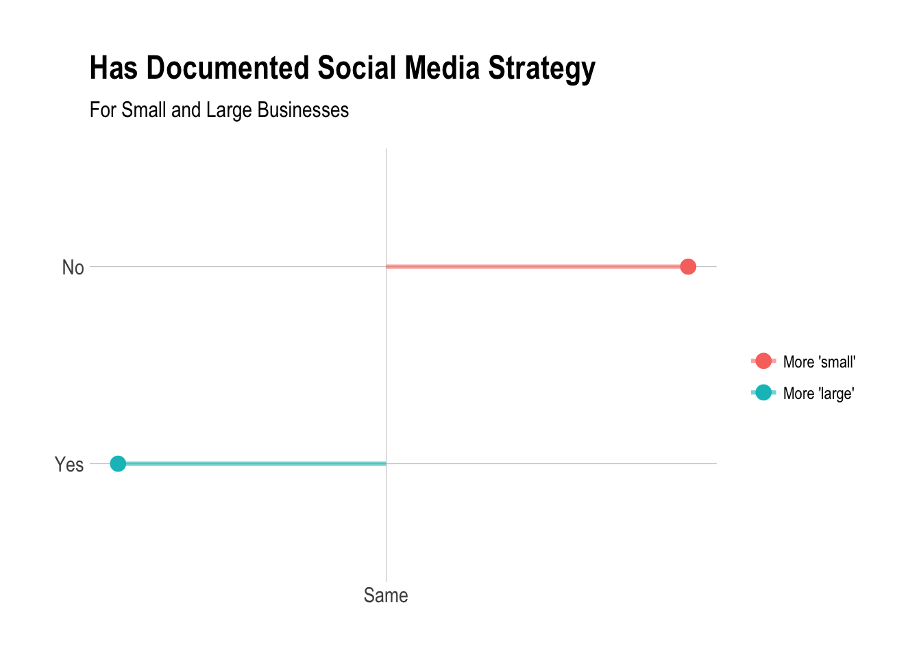
It looks like large businesses are slightly more likely to have a documented social media strategy.
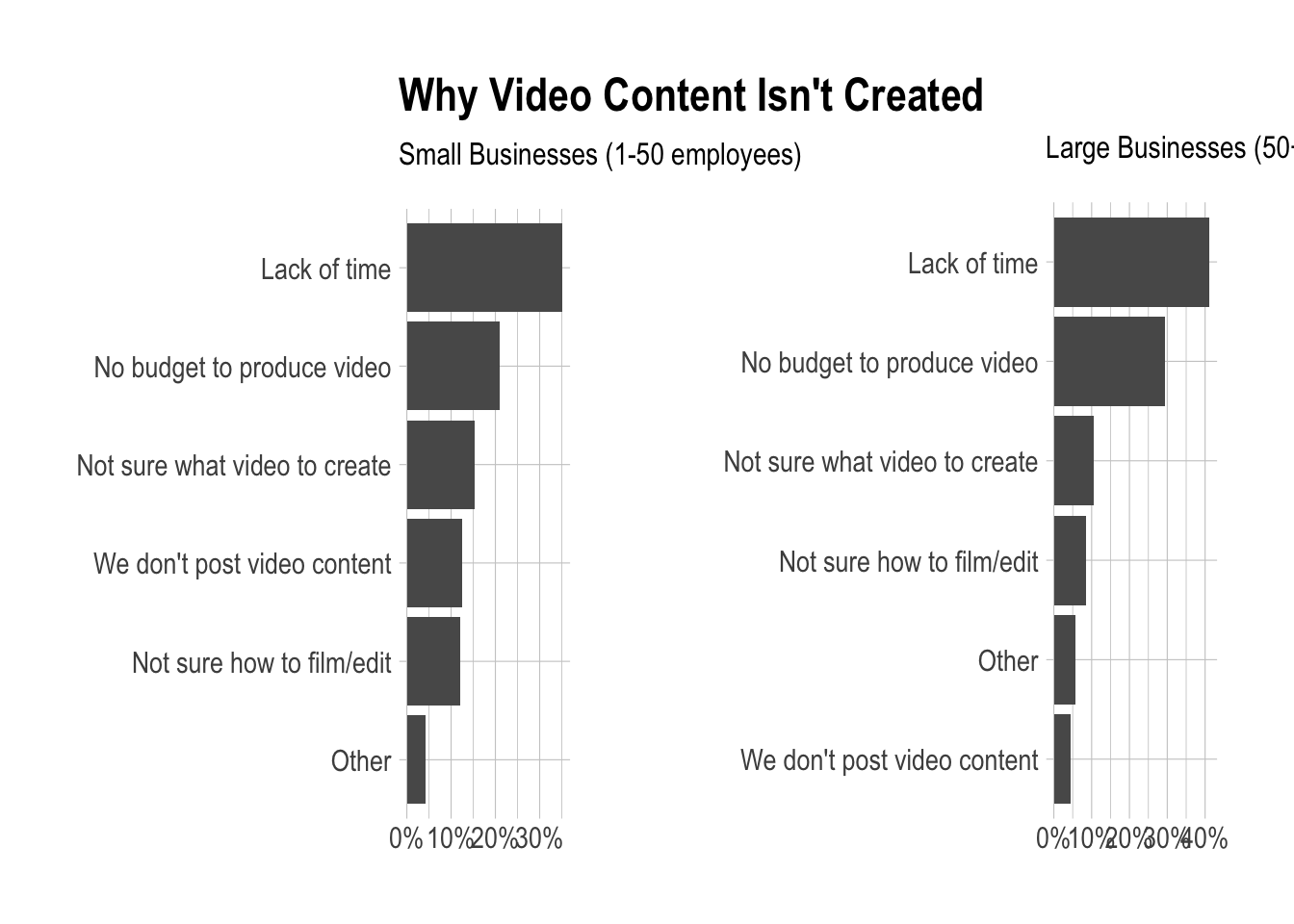
What factors are holding small businesses back from creating video content?
We’ll use the same approach as in the previous two questions. The question numbers are 32-38. This will take some data tidying first. We’ll need to count the number of users that reqponded to each question and bind them into a single data frame.
# get counts for each response
dont_post <- responses %>%
  select(user_id, size, q32) %>%
  rename(reason = q32) %>%
  filter(reason == "We don't post video content")

other <- responses %>%
  select(user_id, size, q33) %>%
  rename(reason = q33) %>%
  filter(reason == "Other")

time <- responses %>%
  select(user_id, size, q34) %>%
  rename(reason = q34) %>%
  filter(reason == "Lack of time")

budget <- responses %>%
  select(user_id, size, q35) %>%
  rename(reason = q35) %>%
  filter(reason == "No budget to produce video")

film <- responses %>%
  select(user_id, size, q36) %>%
  rename(reason = q36) %>%
  filter(reason == 'Not sure how to film/edit')

what <- responses %>%
  select(user_id, size, q37) %>%
  rename(reason = q37) %>%
  filter(reason == 'Not sure what video to create')

by_reason <- dont_post %>%
  bind_rows(other) %>%
  bind_rows(time) %>%
  bind_rows(budget) %>%
  bind_rows(film) %>%
  bind_rows(what)
Now let’s create a side-by-side plot.
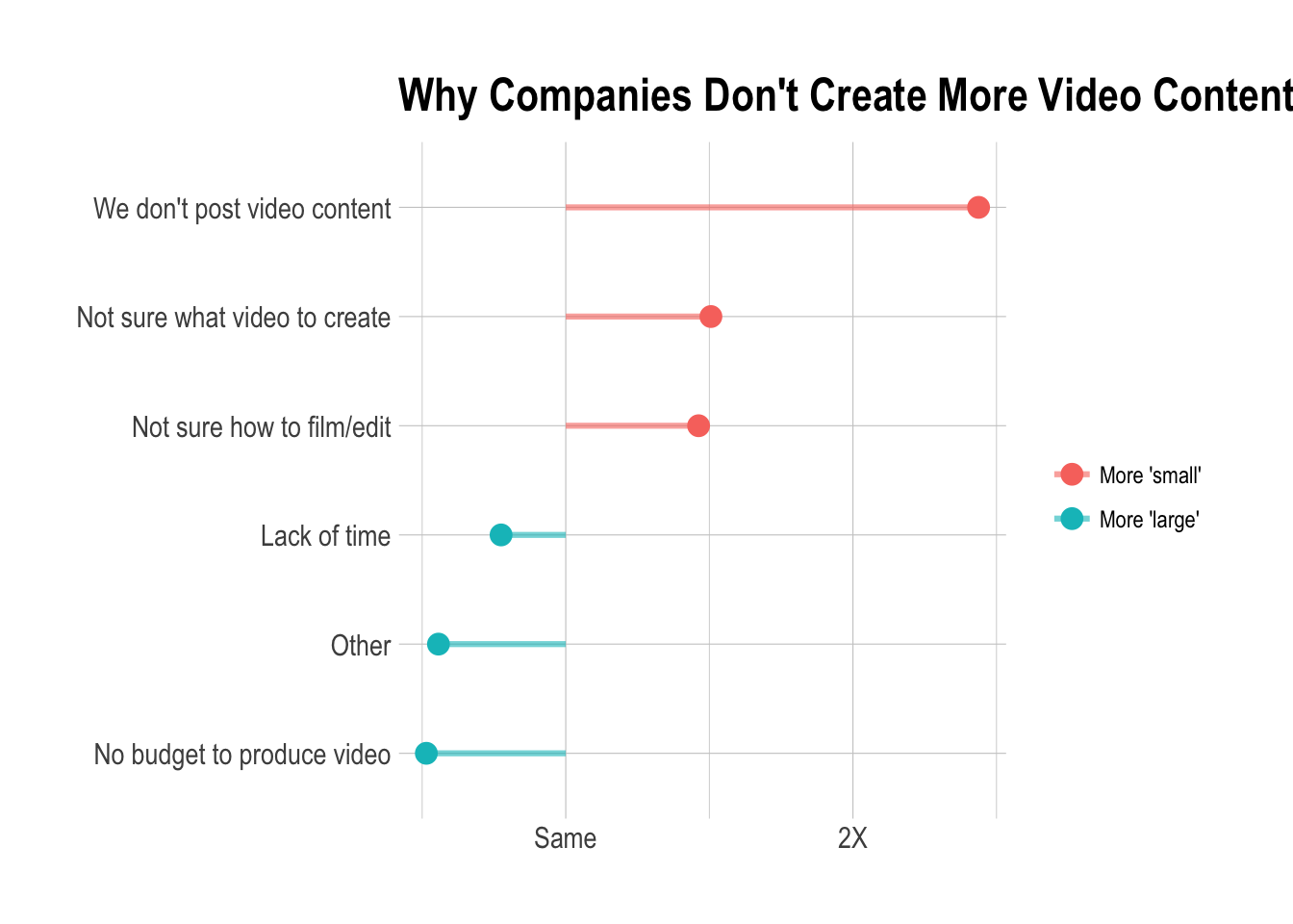
Measuring ROI
Let’s take the same approach to see if there is any difference in how small and large companies measure ROI.
# small business plot
small <- responses %>%
  filter(q74 != '' & size == 'small') %>%
  group_by(q74) %>%
  summarise(n = n_distinct(user_id)) %>%
  mutate(percent = n / sum(n)) %>%
  mutate(q74 = reorder(q74, n)) %>%
  ggplot(aes(x = q74, y = percent)) +
  geom_bar(stat = 'identity') +
  scale_y_continuous(labels = percent) +
  coord_flip() +
  theme_ipsum() +
  labs(x = NULL, y = NULL, title = "How Social Media ROI is Measured",
       subtitle = "Small Businesses (1-50 employees)")

# large business plot
large <- responses %>%
  filter(q74 != '' & size == 'large') %>%
  group_by(q74) %>%
  summarise(n = n_distinct(user_id)) %>%
  mutate(percent = n / sum(n)) %>%
  mutate(q74 = reorder(q74, n)) %>%
  ggplot(aes(x = q74, y = percent)) +
  geom_bar(stat = 'identity') +
  scale_y_continuous(labels = percent) +
  coord_flip() +
  theme_ipsum() +
  labs(x = NULL, y = NULL, title = "",
       subtitle = "Large Businesses (50+ employees)")

# plot two plots together
grid.arrange(small, large, nrow = 1)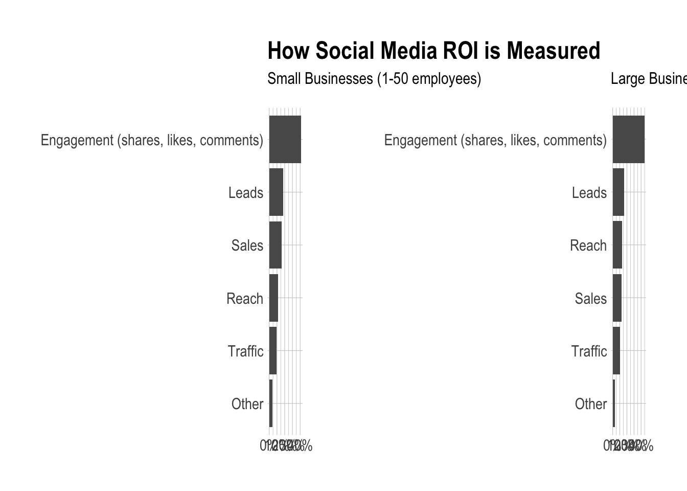
Now let’s plot the log ratios.
roi <- responses %>%
  select(size, q74) %>%
  filter(q74 != '') %>%
  mutate(q74 = as.character(q74))

engagement_rows <- grep("Engagement", roi$q74)
roi[engagement_rows, ]$q74 <- "Engagement"

# calculate log ratios for the counts
counts <- roi %>%
  filter(q74 != '') %>%
  count(size, q74) %>%
  spread(size, n, fill = 0) %>%
  mutate(total = small + large,
         small = (small) / sum(small + 1),
         large = (large + 1) / sum(large + 1),
         log_ratio = log2(small / large),
         abs_ratio = abs(log_ratio)) %>%
  arrange(desc(log_ratio))

# plot the ratios
counts %>%
    group_by(direction = ifelse(log_ratio < 0, 'More "small"', "More 'large'")) %>%
    top_n(15, abs_ratio) %>%
    ungroup() %>%
    mutate(q74 = reorder(q74, log_ratio)) %>%
    ggplot(aes(q74, log_ratio, color = direction)) +
    geom_segment(aes(x = q74, xend = q74,
                     y = 0, yend = log_ratio),
                 size = 1.1, alpha = 0.6) +
    geom_point(size = 3.5) +
    coord_flip() +
    theme_ipsum() +
    labs(x = NULL,
         y = NULL,
         title = "How ROI is Measured",
         subtitle = "For Small and Large Businesses") +
    scale_color_discrete(name = "", labels = c("More 'small'", "More 'large'")) +
    scale_y_continuous(breaks = seq(-3, 3),
                       labels = c("8X", "4X", "2X",
                                  "Same", "2X", "4X", "8X"))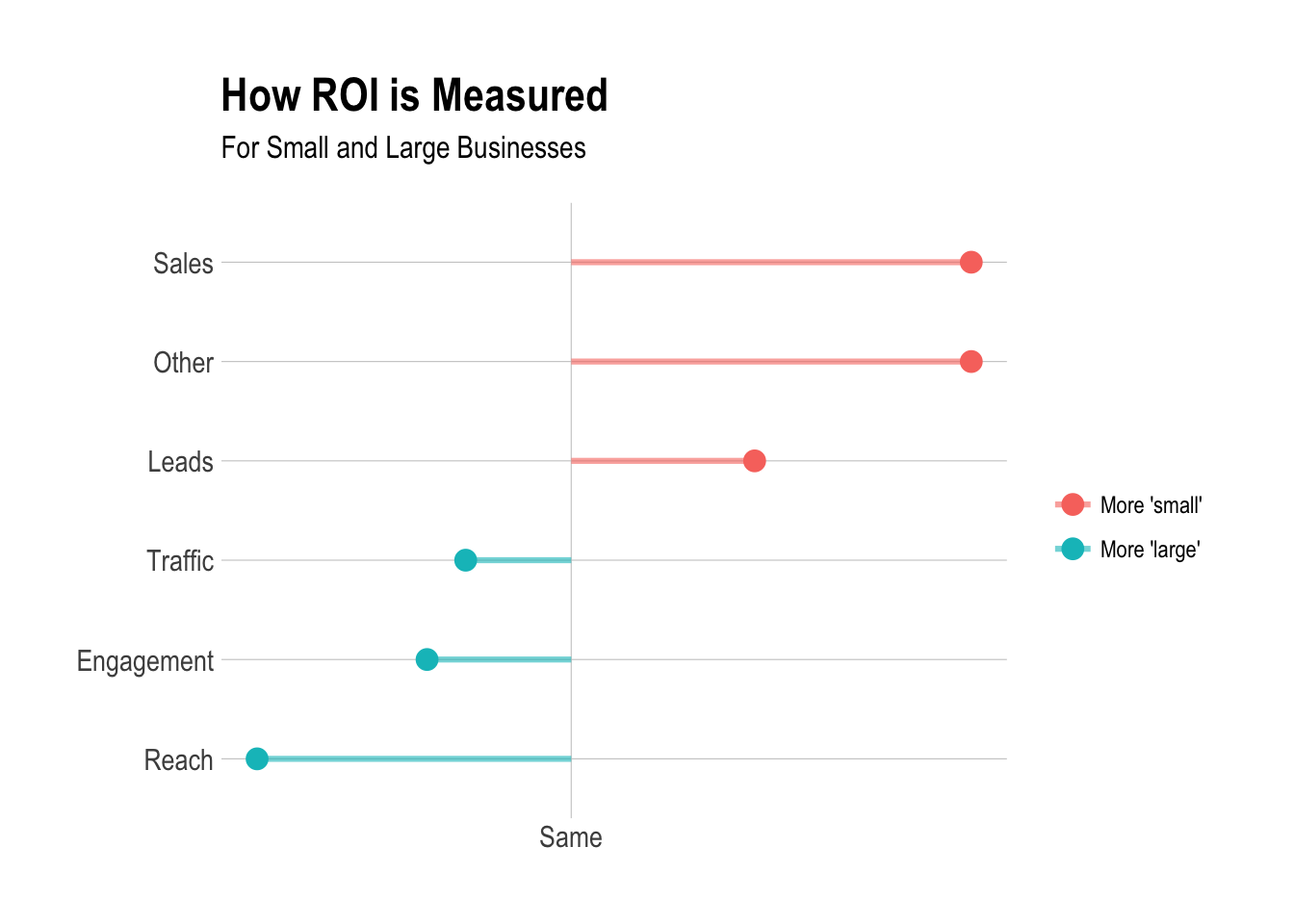
Do people that invest in social media ads see social media marketing as more effective?
People answered questions 66 through 71 with networks in which they’ve invested money in paid advertising. We’ll need to get the user_ids of each person that has invested in at least one of the networks.
# get counts for each network
fb <- responses %>%
  select(user_id, q66) %>%
  rename(network = q66) %>%
  filter(network == 'Facebook')

twitter <- responses %>%
  select(user_id, q69) %>%
  rename(network = q69) %>%
  filter(network == 'Twitter')

ig <- responses %>%
  select(user_id, q67) %>%
  rename(network = q67) %>%
  filter(network == 'Instagram')

li <- responses %>%
  select(user_id, q70) %>%
  rename(network = q70) %>%
  filter(network == 'LinkedIn')

snap <- responses %>%
  select(user_id, q68) %>%
  rename(network = q68) %>%
  filter(network == 'Snapchat')

youtube <- responses %>%
  select(user_id, q71) %>%
  rename(network = q71) %>%
  filter(network == 'YouTube')

# bind all responses together
all_networks <- fb %>%
  bind_rows(ig) %>%
  bind_rows(twitter) %>%
  bind_rows(li) %>%
  bind_rows(snap) %>%
  bind_rows(youtube)

# determine if user has invested in ads
responses <- responses %>%
  mutate(has_run_ads = user_id %in% all_networks$user_id)
Let’s make a side-by-side plot.
# small business plot
has_run_ads <- responses %>%
  filter(has_run_ads == TRUE & q76 != '') %>%
  group_by(q76) %>%
  summarise(n = n_distinct(user_id)) %>%
  mutate(percent = n / sum(n)) %>%
  mutate(q76 = reorder(q76, n)) %>%
  ggplot(aes(x = q76, y = percent)) +
  geom_bar(stat = 'identity') +
  scale_y_continuous(labels = percent) +
  coord_flip() +
  theme_ipsum() +
  labs(x = NULL, y = NULL, title = "Efficacy of Social Media Marketing",
       subtitle = "Companies that have run ads")

# large business plot
not_run_ads <- responses %>%
  filter(has_run_ads == FALSE & q76 != '') %>%
  group_by(q76) %>%
  summarise(n = n_distinct(user_id)) %>%
  mutate(percent = n / sum(n)) %>%
  mutate(q76 = reorder(q76, n)) %>%
  ggplot(aes(x = q76, y = percent)) +
  geom_bar(stat = 'identity') +
  scale_y_continuous(labels = percent) +
  coord_flip() +
  theme_ipsum() +
  labs(x = NULL, y = NULL, title = "",
       subtitle = "Companies that have not run ads")

# plot two plots together
grid.arrange(has_run_ads, not_run_ads, nrow = 1)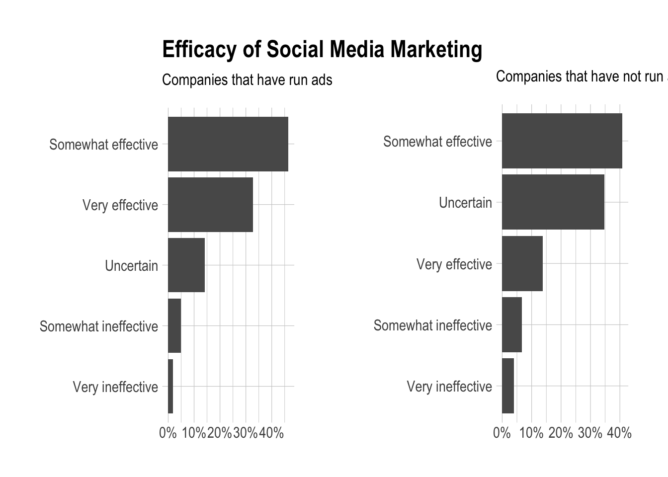
Now let’s see if these users responded any differently to the question about how effective social media marketing is.
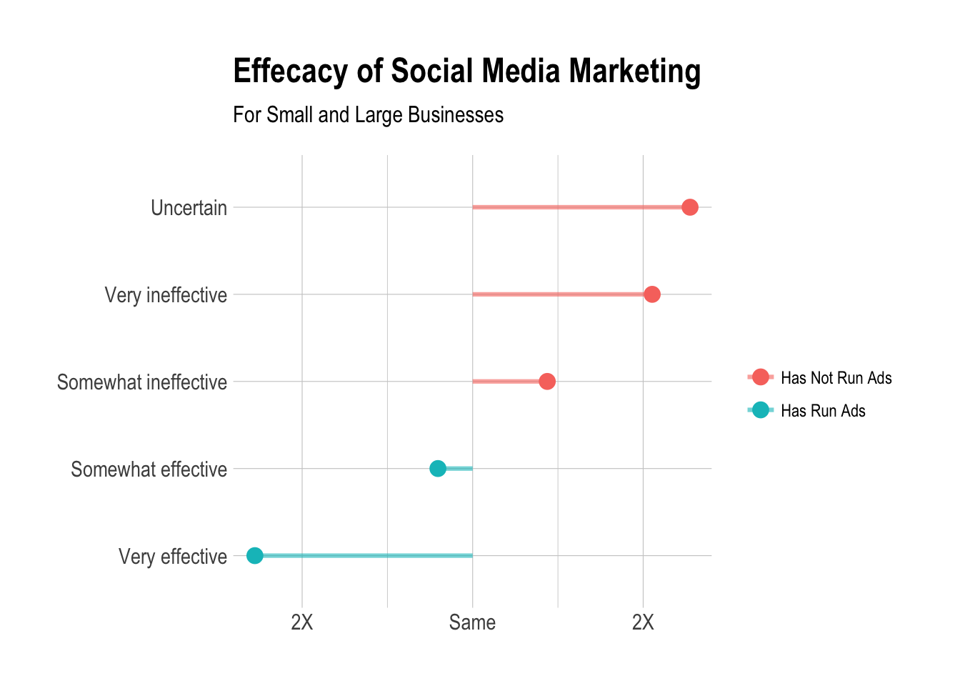
Pretty cool!
responses %>%
  group_by(has_run_ads, q76) %>%
  summarise(users = n_distinct(user_id)) %>%
  mutate(percent = users / sum(users))
## # A tibble: 12 x 4
## # Groups: has_run_ads [2]
## has_run_ads q76 users percent
## <lgl> <fctr> <int> <dbl>
## 1 FALSE 24 0.068181818
## 2 FALSE Somewhat effective 134 0.380681818
## 3 FALSE Somewhat ineffective 22 0.062500000
## 4 FALSE Uncertain 114 0.323863636
## 5 FALSE Very effective 45 0.127840909
## 6 FALSE Very ineffective 13 0.036931818
## 7 TRUE 5 0.003484321
## 8 TRUE Somewhat effective 664 0.462717770
## 9 TRUE Somewhat ineffective 69 0.048083624
## 10 TRUE Uncertain 202 0.140766551
## 11 TRUE Very effective 469 0.326829268
## 12 TRUE Very ineffective 26 0.018118467