Game of Thrones Book Analysis

Winter is here. Finally!

I was inspired by this series of blog posts from the Looker team to do my own Game of Thrones inspired data analysis. While Looker’s analysis focuses on the screentime of different characters in the show, I thought it would be interesting to take a different approach and analyze the text corpuses of the George R. R. Martin’s books.

I was particularly inspired by Julia Silge’s analysis of gender roles in Jane Austen’s works, and took a similar approach to exploring the Game of Thrones data.

We will look at the words that are most closely associated with gendered pronouns like “he” and “she” to try to gain a better understanding of how men and women are portrayed in the series.

Julia Silge and David Robinson’s tidytext package is leaned on heavily in this analysis, as is Stanford’s CoreNLP library for natual language processing. Shall we begin?

Data collection

We begin with five txt files containing the text of the first five novels. To read the data into R, we’ll read in each text file with the readLines() function and bind them into a single dataframe.

# Initialize data frame
df <- tibble()

# Read data
for (i in 1:5) {
  
  # Read text files
  assign(paste0("book", i), readLines(paste0("/Users/julianwinternheimer/Documents/GoT/got", i, ".txt")))
  
  # Create dataframes
  assign(paste0("book", i), tibble(get(paste0("book", i))))
  
  # Bind to the original dataframe
  df <- rbind(df, get(paste0("book", i)))

}

We now have the text of the books in a single dataframe. Let’s clean it up by removing lines in which there is no text.

# Column names
colnames(df) <- 'text'

# Remove rows that are empty
df <- df %>% filter(text != "")

Tidy the text

Here is some context on the idea of tidy data taken from the book Tidy Text Mining with R:

Using tidy data principles is a powerful way to make handling data easier and more effective, and this is no less true when it comes to dealing with text. As described by Hadley Wickham (Wickham 2014), tidy data has a specific structure: - Each variable is a column - Each observation is a row - Each type of observational unit is a table

To get our data into a tidy format, we need each value, or token, to have its own row. We can use the unnest_tokens() function to do this for us. We will end up with a dataframe in which there is one word (token) per row. Associations with the word, like the book or line in which it appeared, would be preserved.

# Unnest the tokens
text_df <- df %>%
  unnest_tokens(word, text)

# Check it out
head(text_df)

## # A tibble: 6 x 1
##      word
##     <chr>
## 1       a
## 2    game
## 3      of
## 4 thrones
## 5       a
## 6    song

Now we want to remove words like “a” and “the” that appear frequently but don’t provide much contextual value. We’ll remove these stop words by “anti-joining” them with our tidy data frame, thus making sure that all stop words are excluded.

# Get stop words
data(stop_words)

# Anti join stop words
text_df <- text_df %>%
  anti_join(stop_words, by = "word")

Alright. Let’s list and visualize the most frequently occuring words in the Game of Thrones books.

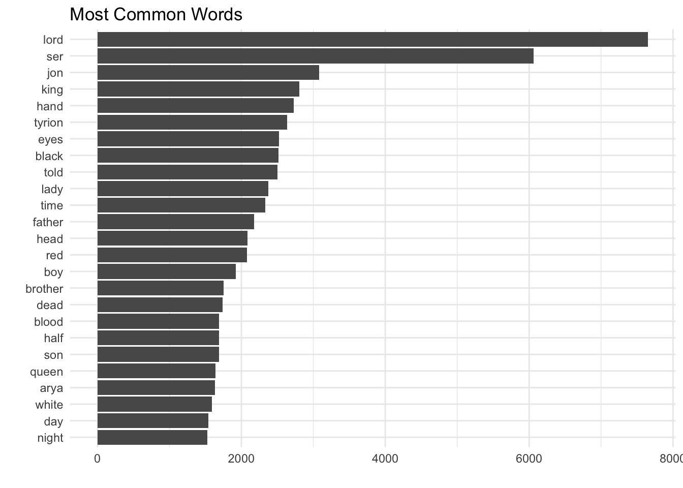
We can see that titles like “lord”, “ser”, and “king”, and names occur most frequently. The frequent occurrence of words like “dead”, “blood” gives us a sense of the violence that these works contain.

We still don’t have a great understanding of the context in which these words occur. One way we can address this is by finding and analyzing groups of words that occur together, i.e. n-grams.

N-grams

An n-gram is a contiguous series of n words from a text; for example, a bigram is a pair of words, with n = 2.

We will use the unnest_tokens function from the tidytext package to identify groups of words that tend to occur together in the books. When we set n to 2, we are examining pairs of two consecutive words, often called “bigrams”.

# Get bigrams
got_bigrams <- df %>%
  unnest_tokens(bigram, text, token = "ngrams", n = 2)

Now that we have our n-grams, we can visualize the most popular ones.

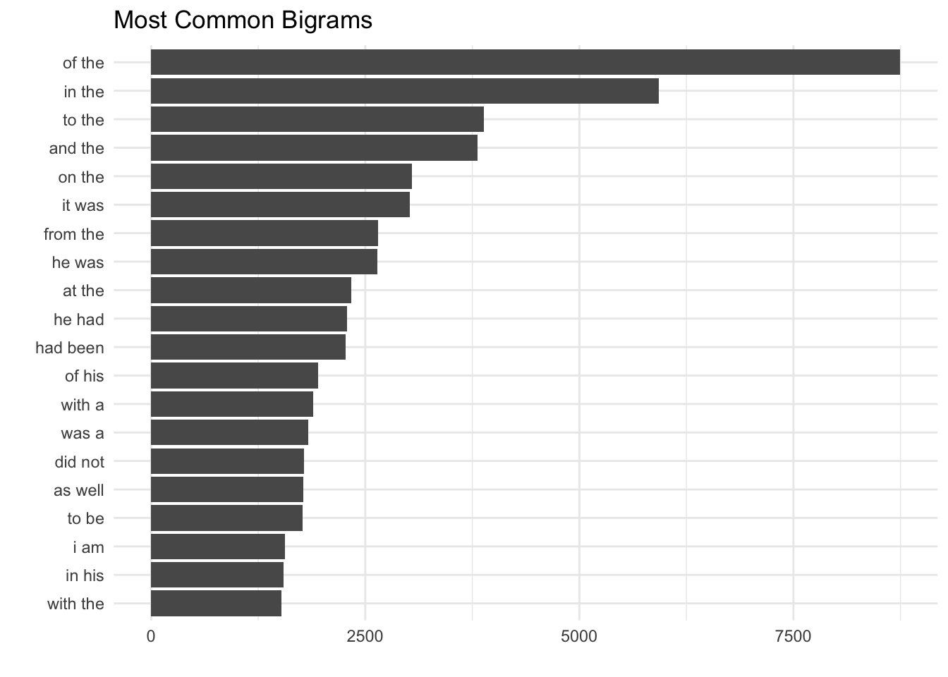
This list is full of stopwords that don’t give us value. We can remove them by separating the two words in the bigram, removing stopwords, and reuniting the words into bigrams.

library(tidyr)

## Warning: package 'tidyr' was built under R version 3.4.1

# Separate the two words
bigrams_separated <- got_bigrams %>%
  separate(bigram, c("word1", "word2"), sep = " ")

# Filter out stopwords
bigrams_filtered <- bigrams_separated %>%
  filter(!word1 %in% stop_words$word) %>%
  filter(!word2 %in% stop_words$word)

# Count the new bigrams
bigram_counts <- bigrams_filtered %>% 
  count(word1, word2, sort = TRUE)

# Unite the bigrams to form words
bigrams_united <- bigrams_filtered %>%
  unite(bigram, word1, word2, sep = " ")

Now we can plot the most common bigrams, excluding stopwords.

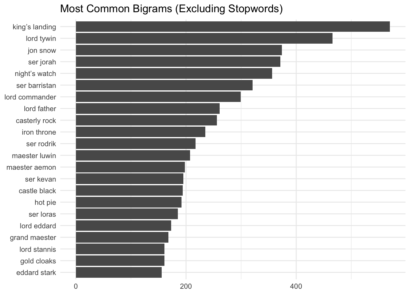
Most of these bigrams are titles or names, which is similar to what we saw when we visualized the most frequently occuring individual words. Also, hot pie. :)

Gendered verbs

This study by Matthew Jockers and Gabi Kirilloff utilizes text mining to examine 19th century novels and explore how gendered pronouns like he/she/him/her are associated with different verbs.

These researchers used the Stanford CoreNLP library to parse dependencies in sentences and find which verbs are connected to which pronouns, but we can also use a tidytext approach to find the most commonly-occuring verbs that appear after these gendered pronouns. The two pronouns we’ll examine here are “he” and “she”.

We can identify these “gendered” bigrams by finding all bigrams in which the first word is “he” or “she”.

# Define our pronouns
pronouns <- c("he", "she")

# Get our bigram where first word is a pronoun
gender_bigrams <- got_bigrams %>%
    count(bigram, sort = TRUE) %>%
    separate(bigram, c("word1", "word2"), sep = " ") %>%
    filter(word1 %in% pronouns) %>%
    count(word1, word2, wt = n, sort = TRUE) %>%
    rename(total = nn)

Let’s visualize the most common gendered bigrams.

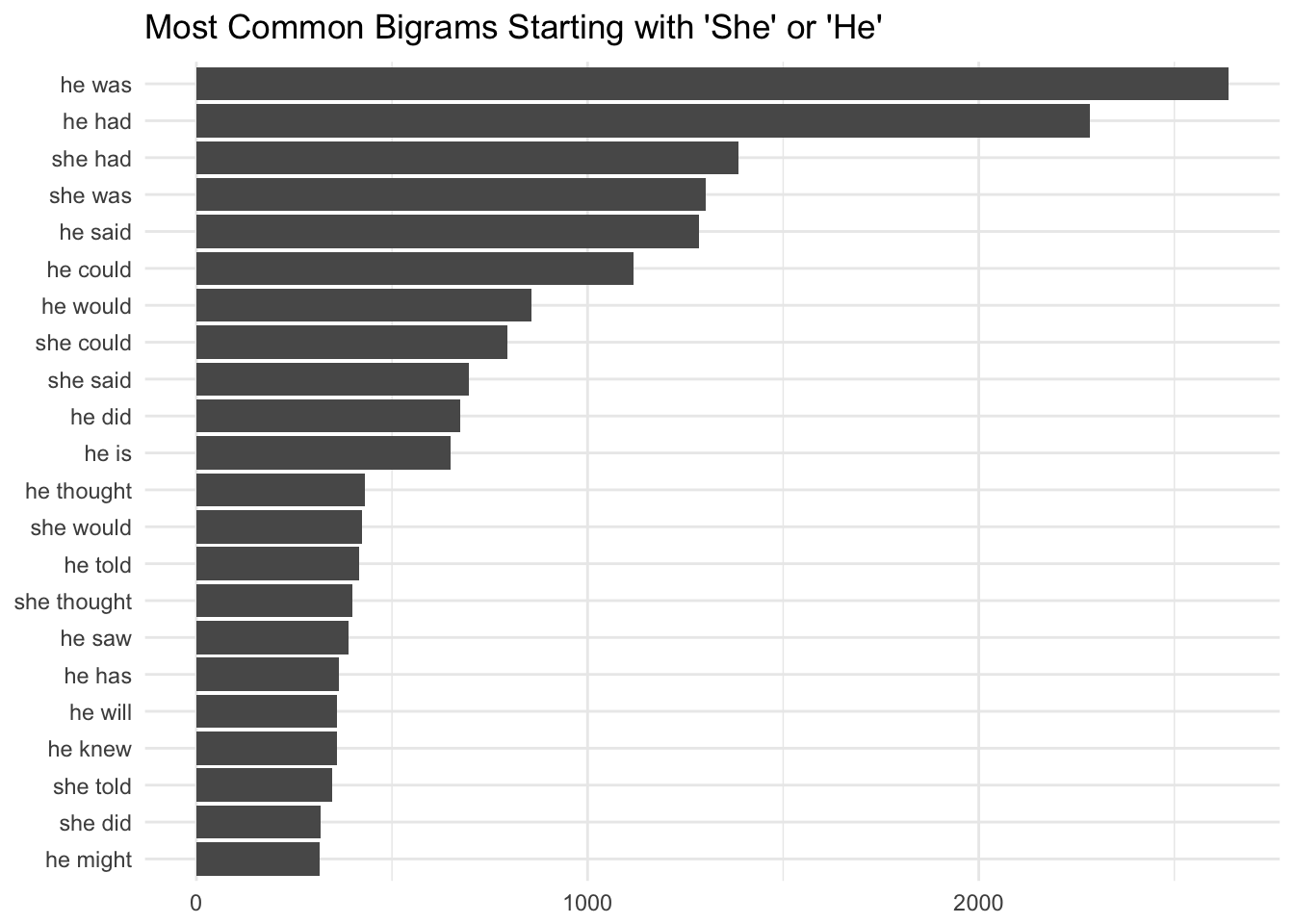
These are the most common bigrams that start with “he” and “she” in the Game of Thrones series. The most common bigrams are similar between the male and female characters.

We can take a different approach and calculate the log odds ratio of words related to “he” and “she”. This will help us find the words that exhibit the biggest differences between relative use after our gendered pronouns.

# Calculate log odds ratio
word_ratios <- gender_bigrams %>%
    group_by(word2) %>%
    filter(sum(total) > 50) %>%
    ungroup() %>%
    spread(word1, total, fill = 0) %>%
    mutate_if(is.numeric, funs((. + 1) / sum(. + 1))) %>%
    mutate(logratio = log2(she / he)) %>%
    arrange(desc(logratio))

Which words have about the same likelihood of following “she” or “he” in the series?

# Arrange by logratio
word_ratios %>% 
    arrange(abs(logratio))

## # A tibble: 117 x 4
##      word2          he         she     logratio
##      <chr>       <dbl>       <dbl>        <dbl>
##  1  caught 0.001656759 0.001662001  0.004558188
##  2     sat 0.003995712 0.004023793  0.010103468
##  3   found 0.010232921 0.010321903  0.012491048
##  4  looked 0.012035864 0.012246326  0.025009301
##  5   stood 0.004824091 0.004723583 -0.030375602
##  6    said 0.062664458 0.061056683 -0.037498185
##  7   tried 0.007163045 0.007435269  0.053812107
##  8 stopped 0.002095312 0.002011896 -0.058609283
##  9  turned 0.010866387 0.010409377 -0.061988621
## 10 laughed 0.003752071 0.003586424 -0.065141020
## # ... with 107 more rows

Words like “caught”, “sat”, and “found” are about as likely to come after the word “she” as the word “he”. Now let’s look at the words that exhibit the largest differences in appearing after “she” compared to “he”. We can do this by sorting words by the magnitude of the log odds ratio of words.

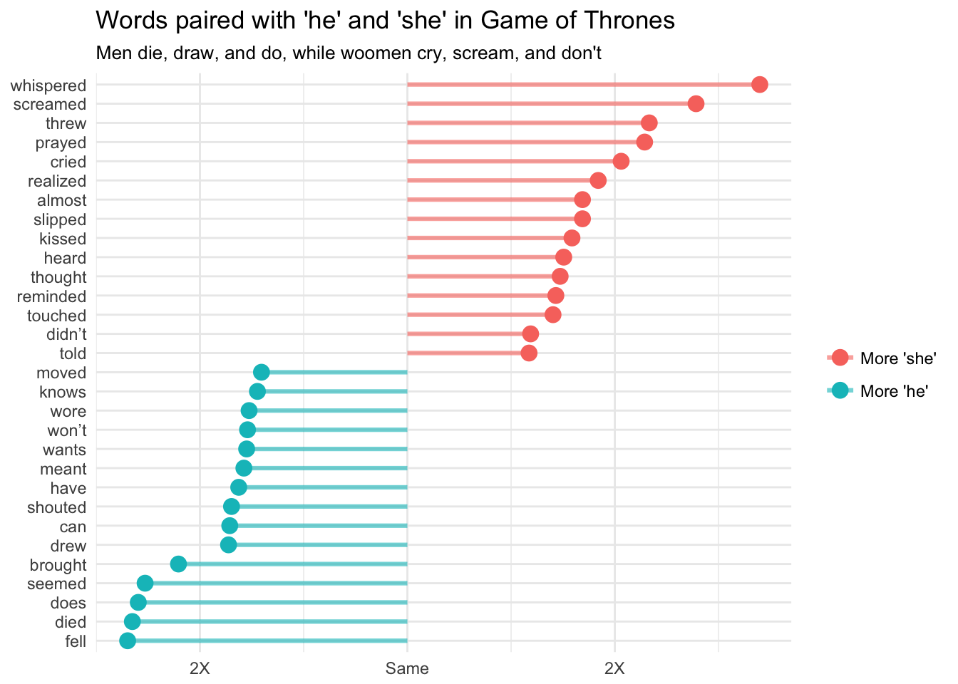
Men are more than twice as likely to fall, die, do, seem, and bring, whereas women are more than twice as likely to whisper, scream, throw, pray, and cry. This doesn’t paint a pretty picture of gender roles in the Game of Thrones series.

More positive, action-oriented verbs like “drew”, “shouted”, “can”, “knows”, and “moved” seem to appear more often for men, while more passive, victim-like verbs like “didn’t”, “screamed”, “slipped”, and “cried” appear more often for women in the series.

The portrayal of women in the Game of Thrones series is a got discussion topic. We also know that certain women in the show and books are portrayed in different ways. Women like Arya might be described by terms more closely resembling those that are associated with the pronoun “he”, whereas other women are not.

We can take advantage of the powerful CoreNLP library to find words that are closely associated with specific characters, regardless of where they appear together in a sentence.

Character dependencies

Let’s use the Stanford CoreNLP library to parse dependencies in sentences and find which verbs are connected to certain proper nouns and pronouns.

# Load library
library(cleanNLP); library(reticulate)

# Setting up NLP backend
init_spaCy()

# Get text
text <- paste(df$text, collapse = " ")

Because our input is a text string we set as_strings to TRUE (the default is to assume that we are giving the function paths to where the input data sits on the local machine“):

obj <- run_annotators(text, as_strings = TRUE)

Here, we used the spaCy backend.The returned annotation object is nothing more than a list of data frames (and one matrix), similar to a set of tables within a database.

Named entities

Named entity recognition is the task of finding entities that can be defined by proper names, categorizing them, and standardizing their formats. Let’s use this approach to get the names of the main characters.

# Find the named entities in our text
people <- get_entity(obj) %>% 
  filter(entity_type == "PERSON" & entity != "Hand" & entity != "Father") %>%
  group_by(entity) %>%
  count %>%
  arrange(desc(n))

# Show the top 20 characters by mention
people[1:20,]

## # A tibble: 20 x 2
## # Groups:   entity [20]
##        entity     n
##         <chr> <int>
##  1        Jon  1826
##  2      Jaime  1195
##  3       Arya   973
##  4       Robb   847
##  5        Sam   800
##  6        Ned   796
##  7     Robert   767
##  8      Sansa   761
##  9       Dany   751
## 10    Catelyn   559
## 11     Cersei   537
## 12    Brienne   522
## 13    "Jon\t"   475
## 14 Your Grace   461
## 15      Grace   348
## 16 Lord Tywin   339
## 17      Stark   339
## 18    Stannis   338
## 19       "\t"   302
## 20     Tyrion   269

Cool! Now that we have the names of the main characters, we can examine the relationship between the names and certain key words.

Dependencies

Dependencies give the grammatical relationship between pairs of words within a sentence. We’ll use the get_dependency() function to find dependencies between words in the books.

# Get the dependencies
dependencies <- get_dependency(obj, get_token = TRUE)

Let’s see at what the dependencies look like.

head(dependencies)

## # A tibble: 6 x 10
##      id   sid   tid tid_target relation relation_full  word lemma
##   <int> <int> <int>      <int>    <chr>         <chr> <chr> <chr>
## 1     1     1     2          1      det          <NA>  GAME  game
## 2     1     1     0          2     ROOT          <NA>  ROOT  ROOT
## 3     1     1     2          3     prep          <NA>  GAME  game
## 4     1     1     3          4     pobj          <NA>    OF    of
## 5     1     1     6          5 compound          <NA>  Song  song
## 6     1     1     2          6    appos          <NA>  GAME  game
## # ... with 2 more variables: word_target <chr>, lemma_target <chr>

The word is related to the target, and the relationship is defined in the relation column. We’re more interested in the lemma and lemma_target as they have been standardized for us. The relationship we’re most interested in is direct dependency (nsubj for nominal subject). Let’s filter the results to show words that are directly dependent on one of our main characters’ names.

# Sub out some names
dependencies$lemma_target <- gsub("daenerys", "dany", dependencies$lemma_target)
dependencies$lemma_target <- gsub("jon snow", "jon", dependencies$lemma_target)

# Find direct dependencies on our main characters
subject_dependencies <- dependencies %>% 
  filter(lemma_target %in% main_characters$entity & relation == 'nsubj') %>%
  group_by(lemma_target, word, relation) %>%
  count

head(subject_dependencies)

## # A tibble: 6 x 4
## # Groups:   lemma_target, word, relation [6]
##   lemma_target      word relation     n
##          <chr>     <chr>    <chr> <int>
## 1         arya  admitted    nsubj     3
## 2         arya    agreed    nsubj     1
## 3         arya     alive    nsubj     1
## 4         arya  ambushed    nsubj     1
## 5         arya announced    nsubj     1
## 6         arya    answer    nsubj     1

Cool! At this point, we may be interested in seeing words that appear more frequently for certain characters than for others. To do that, we can calculate each term’s inverse document frequency (tdf), defined as:

idf(term) = ln(documents / documents containing term)

A term’s inverse document frequency (idf) decreases the weight for commonly used words and increases the weight for words that are not used very much. This can be combined with term frequency to calculate a term’s tf-idf (the two quantities multiplied together), the frequency of a term adjusted for how rarely it is used.

The idea of tf-idf is to find the important words for the content of each collection of words (words’ relative relating to each character) by decreasing the weight for commonly used words and increasing the weight for words that are not used very much in an entire collection of documents, in this case the text of all of the books.

The bind_tf_idf function takes a tidy text dataset as input with one row per token (word), per document. One column (word here) contains the terms, one column contains the documents (lemma_target here), and the last necessary column contains the counts, how many times each document contains each term (n).

# Calculate td-idf
book_words <- dependencies %>%
  filter(lemma_target %in% main_characters$entity & relation == 'nsubj') %>%
  select(lemma_target, word) %>%
  group_by(lemma_target, word) %>% 
  summarise(n = n()) %>%
  bind_tf_idf(word, lemma_target, n)

Now that we’ve calculated tf-idf for each of our main characters, we can visualize the words that are closely associated with them, relative to the word’s association with the other characters.

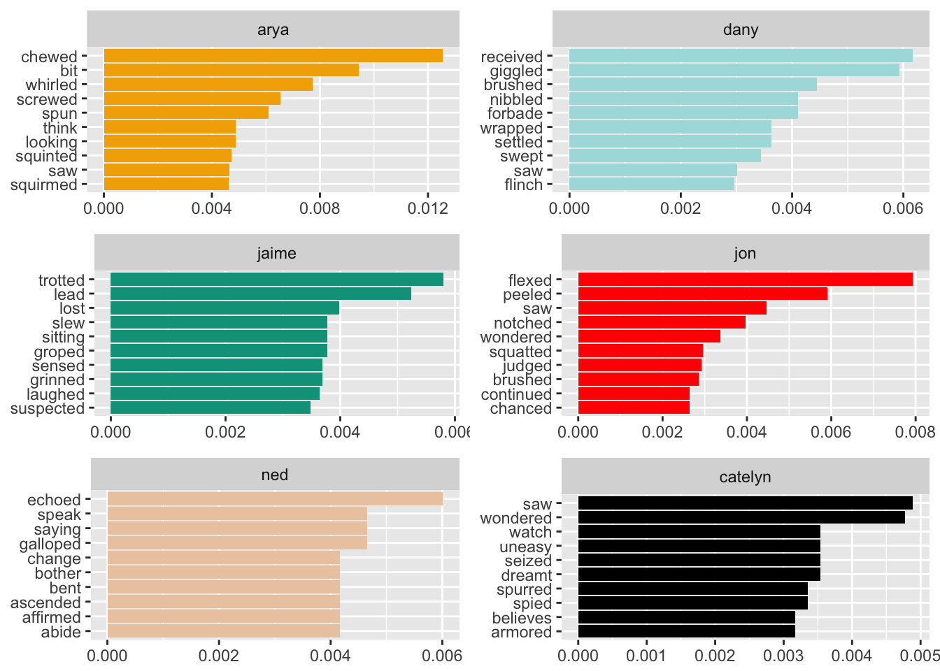
These are fun to see!

Arya is more likely to chew, bite, squirm, and screw.
Dany is more likely to giggle, nibble, grant, forbid, and stroke.
Jaime trots, leads, slays, grins, laughs, and gropes. :(
Jon flexes, notches, judges, squats, and chances.
Ned echoes, speaks, and gallops.
Catelyn sees, watches, and is uneasy.
Robb wins, fights, beats, kills, and dies.
Robert grumbles, dies, commands, swears, and snorts.
Sam stammers, reddens, stresses, puffs, and is uncomfortable. Aw.
Sansa blurts, reddens, cries, drifts, and is anxious.
Cercei paces, weeps, insists, beckons, and does.
Tyrion grins, cocks (?), shrugs, swirls, hops, and reflects.

These main characters have genders, so we can use the same technique as we used above to calculate the log odds ratio for words associated with male or female main characters.

# Get main character words
main_words <- dependencies %>%
  filter(lemma_target %in% named_characters$entity & relation == 'nsubj') %>%
  select(lemma_target, word)

# Join the gender of the main characters
main_words <- main_words %>%
  left_join(named_characters, by = c('lemma_target' = 'entity')) %>%
  filter(word != "’s")

# Calculate log odds ratio
book_words_ratios <- main_words %>%
    group_by(word, gender) %>%
    count %>%
    filter(sum(n) > 10) %>%
    ungroup() %>%
    spread(gender, n, fill = 0) %>%
    mutate_if(is.numeric, funs((. + 1) / sum(. + 1))) %>%
    mutate(logratio = log2(f / m)) %>%
    arrange(desc(logratio))

# Plot word ratios
book_words_ratios %>%
    mutate(abslogratio = abs(logratio)) %>%
    group_by(direction = ifelse(logratio < 0, 'More male', "More female")) %>%
    top_n(10, abslogratio) %>%
    ungroup() %>%
    mutate(word = reorder(word, logratio)) %>%
    ggplot(aes(word, logratio, color = direction)) +
    geom_segment(aes(x = word, xend = word,
                     y = 0, yend = logratio), 
                 size = 1.1, alpha = 0.6) +
    geom_point(size = 3.5) +
    coord_flip() +
    theme_minimal() +
    labs(x = NULL, 
         y = NULL,
         title = "Words Paired with Main Characters",
         subtitle = "Men point, shout, and shrug, while women kiss, blurt, and cry.") +
    scale_color_discrete(name = "", labels = c("More female", "More male")) +
    scale_y_continuous(breaks = seq(-5, 5),
                       labels = c("32X", "16X", "8X", "4X", "2X", 
                                  "Same", "2X", "4X", "8X", "16X", "32X"))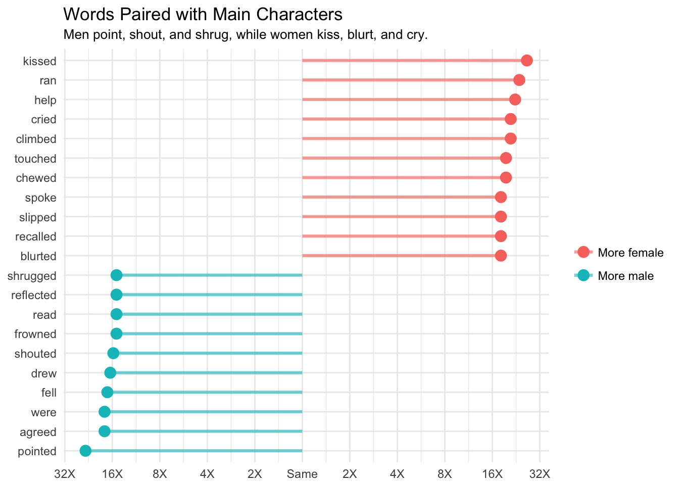

There are some big differences in the relative occurrence of words associated with male and female named characters. I think it’s important to note that we’re working with a relatively small dataset related to 38 named characters. That partially explains why some of the log ratios are so large.

Still, we notice that there are differences in the dependencies of words to characters of different genders. In a future analysis, we can look at how these relative frequencies change for certain characters over the course of the books.

This has been a fun analysis to work on, and I welcome any thoughts or questions!