Churn Prediction with Deep Learning

Preprocessing

We need to do some preprocessing to make the models run more successfully. To do this, we need to do some exploratory data analysis. Let’s begin by taking a look at the seats variable. This represents the quantity of plans that each subscription pays for. An Awesome subscription with two seats is paying for two Awesome plans in a single subscription.

subs %>% 
  group_by(seats, churned) %>% 
  summarise(subs = n_distinct(sub_id)) %>% 
  mutate(percent = subs / sum(subs)) 

## # A tibble: 10 x 4
## # Groups:   seats [7]
##    seats churned  subs    percent
##    <int>   <lgl> <int>      <dbl>
##  1     0   FALSE     1 1.00000000
##  2     1   FALSE 64999 0.91719700
##  3     1    TRUE  5868 0.08280300
##  4     2   FALSE   163 0.95321637
##  5     2    TRUE     8 0.04678363
##  6     3   FALSE    25 1.00000000
##  7     4   FALSE     9 0.90000000
##  8     4    TRUE     1 0.10000000
##  9     5   FALSE     2 1.00000000
## 10     6   FALSE     1 1.00000000

We can see that the vast majority of subscriptions only have one seat. It may not be worth keeping this column as there isn’t enough variability. We’ll also need to remove columns with unique identifiers, such as sub_id and user_id. We do this in the code below.

# remove unnecessary data
churn_data <- subs %>% 
  select(-(sub_id:user_id), -(status:seats), -(created_date:canceled_date))

# glimpse the data
glimpse(churn_data)

## Observations: 75,769
## Variables: 12
## $ plan_id             <fctr> business_v2_small_monthly, pro-annual, pr...
## $ simple_plan_id      <fctr> business, awesome, awesome, awesome, busi...
## $ interval            <fctr> month, year, month, month, year, month, y...
## $ successful_charges  <int> 2, 2, 6, 20, 4, 5, 1, 8, 23, 3, 2, 3, 7, 2...
## $ failed_charges      <int> 0, 0, 0, 5, 3, 0, 0, 0, 0, 0, 0, 0, 3, 5, ...
## $ plan_amount         <int> 99, 102, 10, 10, 1010, 10, 1010, 10, 102, ...
## $ profiles            <int> 2, 10, 5, 16, 2, 12, 4, 6, 10, 34, 0, 4, 2...
## $ updates             <int> 87, 72, 5, 93, 48, 11, 340, 84, 11, 823, 0...
## $ months_since_signup <int> 2, 13, 6, 20, 45, 3, 7, 7, 21, 63, 2, 23, ...
## $ team_members        <dbl> 0, 0, 1, 0, 0, 0, 0, 0, 0, 2, 0, 0, 0, 0, ...
## $ conversations       <dbl> 0, 0, 0, 3, 0, 0, 0, 0, 0, 0, 0, 0, 0, 0, ...
## $ churned             <lgl> FALSE, FALSE, FALSE, FALSE, FALSE, FALSE, ...

Data transformations

The key concept is knowing what transformations are needed to run the algorithm most effectively. Artificial Neural Networks are best when the data is one-hot encoded, scaled and centered. In addition, other transformations may be beneficial as well to make relationships easier for the algorithm to identify.

Let’s look at the charge-related features.

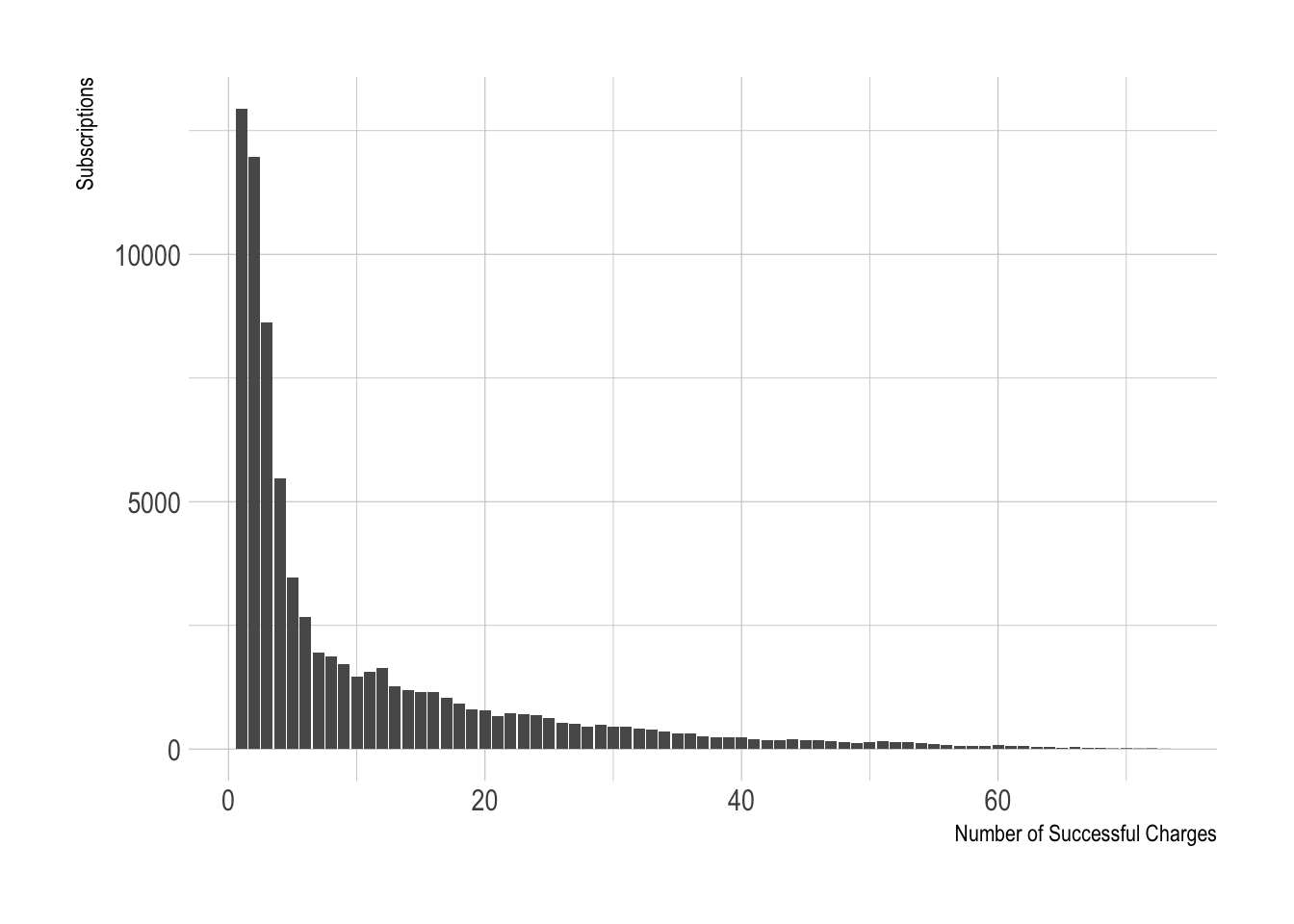
We can see here that there are many values in the low range of number_of_successful_charges. This variable is clearly not scaled and centered. We can apply a log transformation to help with that.

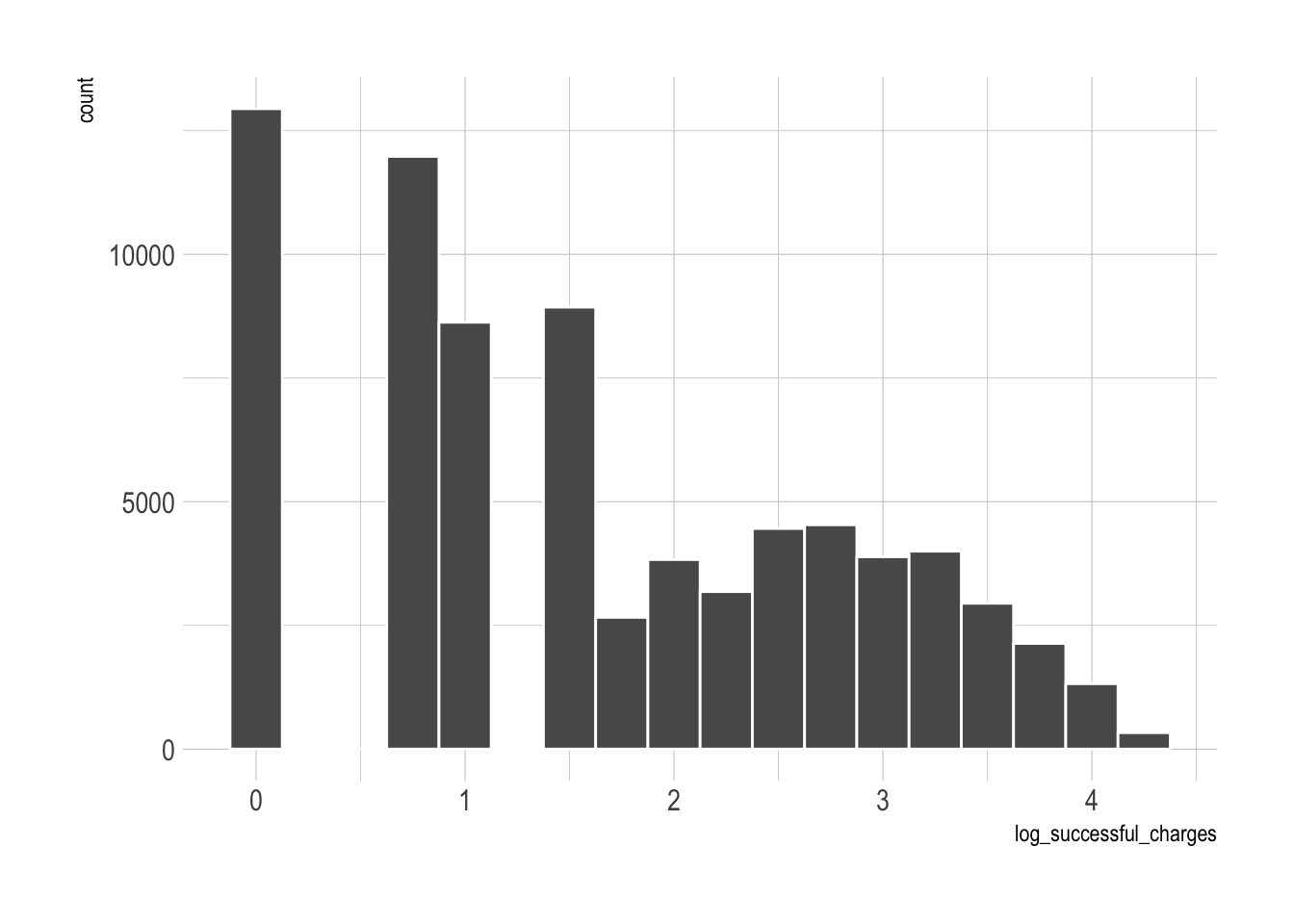
That’s a little better, but not super great. Now let’s look at failed and refunded charges.

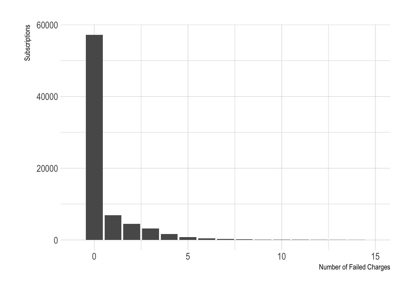
Most subscriptions have 0 failed charges, and we can’t take the log of 0. We could try a square or cube root transformation. But it might be more useful to create a boolean variable indicating whether or not the subscription has had any failed charges.

# see churn rates 
churn_data %>% 
  mutate(has_failed_charge = (failed_charges > 0)) %>% 
  group_by(has_failed_charge, churned) %>% 
  summarise(subs = n()) %>% 
  mutate(percent = subs / sum(subs)) %>% 
  filter(churned == TRUE)

## # A tibble: 2 x 4
## # Groups:   has_failed_charge [2]
##   has_failed_charge churned  subs    percent
##               <lgl>   <lgl> <int>      <dbl>
## 1             FALSE    TRUE  4509 0.07886038
## 2              TRUE    TRUE  1746 0.09391136

We can see that there is a difference in the churn rates of those that have had a failed charge, which is good! Now we create the boolean variable in our data frame.

# create new variables
churn_data <- churn_data %>% 
  filter(!is.na(months_since_signup)) %>% 
  mutate(has_failed_charge = (failed_charges > 0)) %>% 
  select(-failed_charges)

Now let’s look at the months_since_signup variable.

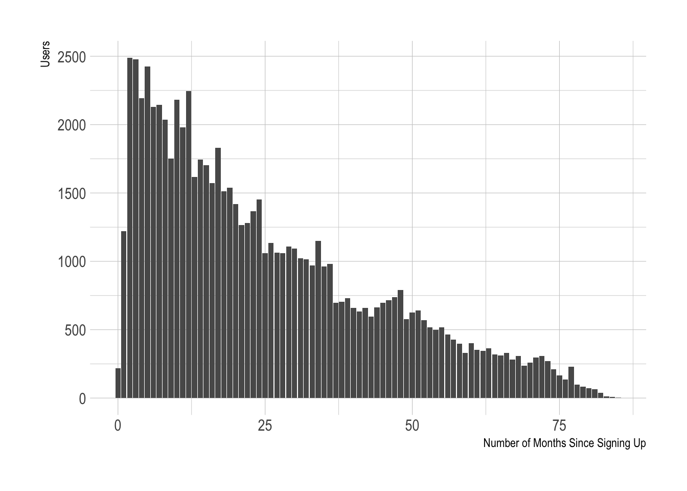
Most of the users with active subscriptions have signed up for Buffer more recently. This makes sense. This feature can be “discretized”, or bucketed, into groups, say of 6-months.

# define breaks
cuts <- seq(0, 85, 6)

# plot new tenure variable
churn_data %>% 
  mutate(tenure = cut(months_since_signup, breaks = cuts)) %>% 
  count(tenure) %>% 
  ggplot(aes(x = tenure, y = n)) +
  geom_bar(stat = 'identity') +
  theme_ipsum() +
  labs(x = "Number of Months Since Signing Up", y = "Users")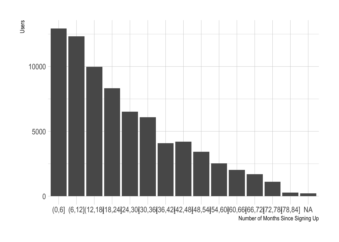

That’s looking better!

Partitioning

Now we’re ready to split the data into training and testing sets. We’ll use the rsample package for this.

# set seed for reproducibility
set.seed(100)

# split data
train_test_split <- initial_split(churn_data, prop = 0.8)

# view split
train_test_split

## <60615/15153/75768>

There are 60,615 subscriptions in the trianing dataset and 15,153 subscriptions in the testing dataset. We can retrieve our training and testing sets using training() and testing() functions.

# retreive the training and testing sets
training <- training(train_test_split)
testing <- testing(train_test_split)

One-hot encoding

One-hot encoding is the process of converting categorical data to sparse data, which has columns of only zeros and ones (this is also called creating “dummy variables” or a “design matrix”). All non-numeric data will need to be converted to dummy variables. This is simple for binary Yes/No data because we can simply convert to 1’s and 0’s. It becomes slightly more complicated with multiple categories, which requires creating new columns of 1’s and 0`s for each value (actually one less).

Recipes

A recipe is a series of steps we would like to perform on the training, testing, and validation datasets. Think of preprocessing data like baking a cake. The recipe explicitly states the steps needed to make the cake. It doesn’t do anything other than list the steps.

We use the recipe() function to implement our preprocessing steps. The function takes a familiar object argument, which is a modeling function such as object = churned ~ . meaning “churned” is the outcome and all other features are predictors. The function also takes the data argument, which gives the recipe steps perspective on how to apply during baking.

A recipe is not very useful until we add steps, which are used to transform the data during baking. The package contains a number of useful step functions that can be applied. For our model, we use:

• step_discretize() with the option = list(cuts = 6) to cut the continuous variable for months_since_signup to group customers into cohorts.
• step_log() to log transform successful_charges.
• step_dummy() to one-hot encode the categorical data. Note that this adds columns of one/zero for categorical data with three or more categories.
• step_center() to mean-center the data.
• step_scale() to scale the data.

The last step is to prepare the recipe with the prep() function. This step is used to “estimate the required parameters from a training set that can later be applied to other data sets”. This is important for centering and scaling and other functions that use parameters defined from the training set.

# create recipe
rec_obj <- recipe(churned ~ ., data = training) %>%
  step_discretize(months_since_signup, options = list(cuts = 6)) %>%
  step_log(successful_charges) %>%
  step_dummy(all_nominal(), -all_outcomes()) %>%
  step_center(all_predictors(), -all_outcomes()) %>%
  step_scale(all_predictors(), -all_outcomes()) %>%
  prep(data = training)

We can print the recipe object if we ever forget what steps were used to prepare the data.

rec_obj

## Data Recipe
## 
## Inputs:
## 
##       role #variables
##    outcome          1
##  predictor         10
## 
## Training data contained 60615 data points and no missing data.
## 
## Operations:
## 
## Dummy variables from months_since_signup [trained]
## Log transformation on successful_charges [trained]
## Dummy variables from simple_plan_id, interval, ... [trained]
## Centering for successful_charges, plan_amount, ... [trained]
## Scaling for successful_charges, plan_amount, ... [trained]

We can apply the recipe to any data set with the bake() function, and it processes the data following our recipe steps. We’ll apply to our training and testing data to convert from raw data to a machine learning dataset. Check our training set out with glimpse(). Now it’s an ML-ready dataset prepared for ANN modeling!

# predictors
x_train_tbl <- bake(rec_obj, newdata = training) %>% select(-churned)
x_test_tbl  <- bake(rec_obj, newdata = testing) %>% select(-churned)

glimpse(x_train_tbl)

## Observations: 60,615
## Variables: 16
## $ successful_charges        <dbl> -0.79506737, 0.13834790, 1.16128076,...
## $ plan_amount               <dbl> 0.05297433, -0.39502380, -0.39502380...
## $ profiles                  <dbl> -0.43928366, -0.25586509, 0.41666965...
## $ updates                   <dbl> -0.02322058, -0.05589073, -0.0208300...
## $ team_members              <dbl> -0.2358782, 0.4313371, -0.2358782, -...
## $ conversations             <dbl> -0.1075231, -0.1075231, 23.3367621, ...
## $ simple_plan_id_business   <dbl> 2.7434270, -0.3645016, -0.3645016, 2...
## $ simple_plan_id_enterprise <dbl> -0.03173876, -0.03173876, -0.0317387...
## $ interval_year             <dbl> -0.8791031, -0.8791031, -0.8791031, ...
## $ months_since_signup_bin1  <dbl> 2.1824067, 2.1824067, -0.4582022, -0...
## $ months_since_signup_bin2  <dbl> -0.4414737, -0.4414737, -0.4414737, ...
## $ months_since_signup_bin3  <dbl> -0.4520486, -0.4520486, 2.2121152, -...
## $ months_since_signup_bin4  <dbl> -0.453900, -0.453900, -0.453900, -0....
## $ months_since_signup_bin5  <dbl> -0.4311598, -0.4311598, -0.4311598, ...
## $ months_since_signup_bin6  <dbl> -0.4462933, -0.4462933, -0.4462933, ...
## $ has_failed_charge_yes     <dbl> -0.5718909, -0.5718909, 1.7485566, 1...

Looky ’dere. One last step, we need to store the actual values (the true observations) as y_train_vec and y_test_vec, which are needed for modeling our ANN. We convert to a series of numeric ones and zeros which can be accepted by the Keras ANN modeling functions. We add vec to the name so we can easily remember the class of the object (it’s easy to get confused when working with tibbles, vectors, and matrix data types).

# response variables for training and testing sets
y_train_vec <- ifelse(pull(training, churned) == "yes", 1, 0)
y_test_vec  <- ifelse(pull(testing, churned) == "yes", 1, 0)

Modeling customer churn

We’re going to build a special class of ANN called a Multi-Layer Perceptron (MLP). MLPs are one of the simplest forms of deep learning, but they are both highly accurate and serve as a jumping-off point for more complex algorithms. MLPs are quite versatile as they can be used for regression, binary and multi classification (and are typically quite good at classification problems).

We’ll build a three layer MLP with Keras. Let’s walk-through the steps before we implement in R.

• Initialize a sequential model: The first step is to initialize a sequential model with keras_model_sequential(), which is the beginning of our Keras model. The sequential model is composed of a linear stack of layers.

• Apply layers to the sequential model: Layers consist of the input layer, hidden layers and an output layer. The input layer is the data and provided it’s formatted correctly there’s nothing more to discuss. The hidden layers and output layers are what controls the ANN inner workings.

• Hidden Layers: Hidden layers form the neural network nodes that enable non-linear activation using weights. The hidden layers are created using layer_dense(). We’ll add two hidden layers. We’ll apply units = 16, which is the number of nodes. We’ll select kernel_initializer = "uniform" and activation = "relu" for both layers. The first layer needs to have the input_shape equal to the number of columns in the training set. Key Point: While we are arbitrarily selecting the number of hidden layers, units, kernel initializers and activation functions, these parameters can be optimized through a process called hyperparameter tuning.

• Dropout Layers: Dropout layers are used to control overfitting. This eliminates weights below a cutoff threshold to prevent low weights from overfitting the layers. We use the layer_dropout() function add two drop out layers with rate = 0.10 to remove weights below 10%.

• Output Layer: The output layer specifies the shape of the output and the method of assimilating the learned information. The output layer is applied using the layer_dense(). For binary values, the shape should be units = 1. For multi-classification, the units should correspond to the number of classes. We set the kernel_initializer = "uniform" and the activation = "sigmoid" (common for binary classification).

Compile the model: The last step is to compile the model with compile(). We’ll use optimizer = "adam", which is one of the most popular optimization algorithms. We select loss = "binary_crossentropy" since this is a binary classification problem. We’ll select metrics = c("accuracy") to be evaluated during training and testing. Key Point: The optimizer is often included in the tuning process.

# building the Artificial Neural Network
model_keras <- keras_model_sequential()

model_keras %>% 
  
  # first hidden layer
  layer_dense(
    units = 16, 
    kernel_initializer = "uniform", 
    activation = "relu", 
    input_shape = ncol(x_train_tbl)) %>% 
  
  # dropout to prevent overfitting
  layer_dropout(rate = 0.1) %>%
  
  # second hidden layer
  layer_dense(
    units = 16, 
    kernel_initializer = "uniform", 
    activation  = "relu") %>% 
  
  # dropout to prevent overfitting
  layer_dropout(rate = 0.1) %>%
  
  # output layer
  layer_dense(
    units = 1, 
    kernel_initializer = "uniform", 
    activation = "sigmoid") %>% 
  
  # compile ANN
  compile(
    optimizer = 'adam',
    loss = 'binary_crossentropy',
    metrics = c('accuracy')
  )

model_keras

## Model
## ___________________________________________________________________________
## Layer (type)                     Output Shape                  Param #     
## ===========================================================================
## dense_1 (Dense)                  (None, 16)                    272         
## ___________________________________________________________________________
## dropout_1 (Dropout)              (None, 16)                    0           
## ___________________________________________________________________________
## dense_2 (Dense)                  (None, 16)                    272         
## ___________________________________________________________________________
## dropout_2 (Dropout)              (None, 16)                    0           
## ___________________________________________________________________________
## dense_3 (Dense)                  (None, 1)                     17          
## ===========================================================================
## Total params: 561
## Trainable params: 561
## Non-trainable params: 0
## ___________________________________________________________________________

Now let’s fit the model to the training data.

# fit the keras model to the training data
history <- fit(
  object = model_keras, 
  x = as.matrix(x_train_tbl), 
  y = y_train_vec,
  batch_size = 50, 
  epochs = 35,
  validation_split = 0.30
)

We can inspect the training history. We want to make sure there is minimal difference between the validation accuracy and the training accuracy.

# print model summary statistics
print(history)

## Trained on 42,430 samples, validated on 18,185 samples (batch_size=50, epochs=35)
## Final epoch (plot to see history):
## val_loss: 0.231
##  val_acc: 0.9357
##     loss: 0.2755
##      acc: 0.9146

Wow, accuracy was quite high, even on the validation set!

We can visualize the Keras training history using the plot() function. What we want to see is the validation accuracy and loss leveling off, which means the model has completed training. We see that there is some divergence between training loss/accuracy and validation loss/accuracy. This model indicates we can possibly stop training at an earlier epoch. Pro Tip: Only use enough epochs to get a high validation accuracy. Once validation accuracy curve begins to flatten or decrease, it’s time to stop training.

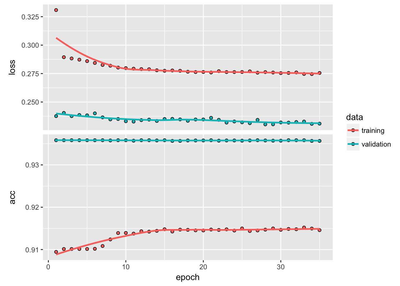
It’ interesting to see that accuracy remains relatively constant throughout training, apart from the first epoch. It may be useful to remember that if we predicted that everyone would churn, we would have a model that achieves 91.8% accuracy.

Making predictions

We’ve got a good model based on the validation accuracy. Now let’s make some predictions from our keras model on the testing set, which was unseen during modeling. We have two functions to generate predictions:

• predict_classes(): Generates class values as a matrix of ones and zeros. Since we are dealing with binary classification, we’ll convert the output to a vector.

• predict_proba(): Generates the class probabilities as a numeric matrix indicating the probability of being a class. Again, we convert to a numeric vector because there is only one column output.

# predicted class
yhat_class_vec <- predict_classes(object = model_keras, x = as.matrix(x_test_tbl)) %>% as.vector()

# predicted class probability
yhat_prob_vec  <- predict_proba(object = model_keras, x = as.matrix(x_test_tbl)) %>% as.vector()

Inspect performance with Yardstick

The yardstick package has a collection of handy functions for measuring performance of machine learning models. We’ll overview some metrics we can use to understand the performance of our model.

First, let’s get the data formatted for yardstick. We create a data frame with the truth (actual values as factors), estimate (predicted values as factors), and the class probability (probability of yes as numeric). We use the fct_recode() function from the forcats package to assist with recoding as Yes/No values.

# format test data and predictions for yardstick metrics
estimates_keras_tbl <- tibble(
  truth      = as.factor(y_test_vec) %>% fct_recode(yes = "1", no = "0"),
  estimate   = as.factor(yhat_class_vec) %>% fct_recode(yes = "1", no = "0"),
  class_prob = yhat_prob_vec
)

head(estimates_keras_tbl, n = 10)

## # A tibble: 10 x 3
##     truth estimate  class_prob
##    <fctr>   <fctr>       <dbl>
##  1     no       no 0.048169497
##  2     no       no 0.015589011
##  3     no       no 0.017783972
##  4     no       no 0.009276078
##  5     no       no 0.108753555
##  6     no       no 0.162961081
##  7     no       no 0.021975949
##  8     no       no 0.016171509
##  9     no       no 0.024991035
## 10     no       no 0.011792799

Now that we have the data formatted, we can take advantage of the yardstick package. The only other thing we need to do is to set options(yardstick.event_first = FALSE), because the default is to classify 0 as the positive class instead of 1.

options(yardstick.event_first = FALSE)

Confusion matrix

We can use the conf_mat() function to get the confusion table. We see that the model was by no means perfect, but it did a decent job of identifying customers likely to churn. It missed a good amount of users that churned, but most of those that were likely to churn did in fact churn.

# confusion matrix
estimates_keras_tbl %>% conf_mat(truth, estimate)

##           Truth
## Prediction    no   yes
##        no  13836  1208
##        yes    42    67

We can use the metrics() function to get an accuracy measurement from the test set. We are getting roughly 92% accuracy. Probably because most folks do not churn.

# get accuracy
estimates_keras_tbl %>% metrics(truth, estimate)

## # A tibble: 1 x 1
##    accuracy
##       <dbl>
## 1 0.9175081

We can also get the ROC Area Under the Curve (AUC) measurement. AUC is often a good metric used to compare different classifiers and to compare to randomly guessing (AUC_random = 0.50). Our model has AUC = 0.70, which is better than randomly guessing. Tuning and testing different classification algorithms may yield even better results.

# get AUC
estimates_keras_tbl %>% roc_auc(truth, class_prob)

## [1] 0.7056872

We can also calculate precision and recall. Precision is when the model predicts “yes”, how often is it actually “yes”. Recall (also true positive rate or specificity) is when the actual value is “yes” how often is the model correct. In our case, I think we would like to optimize for recall.

# precision and recall
tibble(
  precision = estimates_keras_tbl %>% precision(truth, estimate),
  recall = estimates_keras_tbl %>% recall(truth, estimate)
)

## # A tibble: 1 x 2
##   precision     recall
##       <dbl>      <dbl>
## 1 0.6146789 0.05254902

Precision and recall are very important to the business case: The organization is concerned with balancing the cost of targeting and retaining customers at risk of leaving with the cost of inadvertently targeting customers that are not planning to leave (and potentially decreasing revenue from this group). The threshold above which to predict Churn = “Yes” can be adjusted to optimize for the business problem.

Explaining the model with LIME

LIME stands for Local Interpretable Model-agnostic Explanations, and is a method for explaining black-box machine learning model classifiers. The lime package implements LIME in R. We’ll need to make two custom functions:

• model_type: Used to tell lime what type of model we are dealing with. It could be classification, regression, survival, etc.

• predict_model: Used to allow lime to perform predictions that its algorithm can interpret.

The first thing we need to do is identify the class of our model object. We do this with the class() function.

class(model_keras)

## [1] "keras.models.Sequential"         "keras.engine.training.Model"    
## [3] "keras.engine.topology.Container" "keras.engine.topology.Layer"    
## [5] "python.builtin.object"

Next we create our model_type() function. It’s only input is x the keras model. The function simply returns “classification”, which tells LIME we are classifying.

# setup lime::model_type() function for keras
model_type.keras.models.Sequential <- function(x, ...) {
  "classification"
}

Now we can create our predict_model() function, which wraps keras::predict_proba(). The trick here is to realize that it’s inputs must be x a model, newdata a dataframe object (this is important), and type which is not used but can be use to switch the output type. The output is also a little tricky because it must be in the format of probabilities by classification (this is important; shown next).

# setup lime::predict_model() function for keras
predict_model.keras.models.Sequential <- function(x, newdata, type, ...) {
  pred <- predict_proba(object = x, x = as.matrix(newdata))
  data.frame(Yes = pred, No = 1 - pred)
}

Run this next script to show you what the output looks like and to test our predict_model() function. See how it’s the probabilities by classification. It must be in this form for model_type = "classification".

# test our predict_model() function
predict_model(x = model_keras, newdata = x_test_tbl, type = 'raw') %>%
  tibble::as_tibble()

## # A tibble: 15,153 x 2
##            Yes        No
##          <dbl>     <dbl>
##  1 0.048169497 0.9518305
##  2 0.015589011 0.9844110
##  3 0.017783972 0.9822160
##  4 0.009276078 0.9907239
##  5 0.108753555 0.8912464
##  6 0.162961081 0.8370389
##  7 0.021975949 0.9780241
##  8 0.016171509 0.9838285
##  9 0.024991035 0.9750090
## 10 0.011792799 0.9882072
## # ... with 15,143 more rows

Now we create an explainer using the lime() function. Just pass the training data set without the “Attribution column”. The form must be a data frame, which is OK since our predict_model function will switch it to an keras object. Set model = automl_leader our leader model, and bin_continuous = FALSE. We could tell the algorithm to bin continuous variables, but this may not make sense for categorical numeric data that we didn’t change to factors.

# run lime() on training set
explainer <- lime::lime(
  x = x_train_tbl, 
  model = model_keras, 
  bin_continuous = FALSE
)

Now we run the explain() function, which returns our explanation. This can take a minute to run so we limit it to just the first ten rows of the test data set. We set n_labels = 1 because we care about explaining a single class. Setting n_features = 4 returns the top four features that are critical to each case. Finally, setting kernel_width = 0.5 allows us to increase the “model_r2” value by shrinking the localized evaluation.

# run explain() on explainer
explanation <- lime::explain(
  x_test_tbl[1:10, ], 
  explainer = explainer, 
  n_labels = 1, 
  n_features = 4,
  kernel_width = 0.5
)

Feature importance visualization

The payoff for the work we put in using LIME is this feature importance plot. This allows us to visualize each of the first ten cases (observations) from the test data. The top four features for each case are shown. Note that they are not the same for each case. The green bars mean that the feature supports the model conclusion, and the red bars contradict. A couple important features based on frequency in first ten cases:

• months_since_signup (8 cases)
• updates(9 cases)

plot_features(explanation) +
  labs(title = "LIME Feature Importance Visualization",
       subtitle = "Hold Out (Test) Set, First 10 Cases Shown")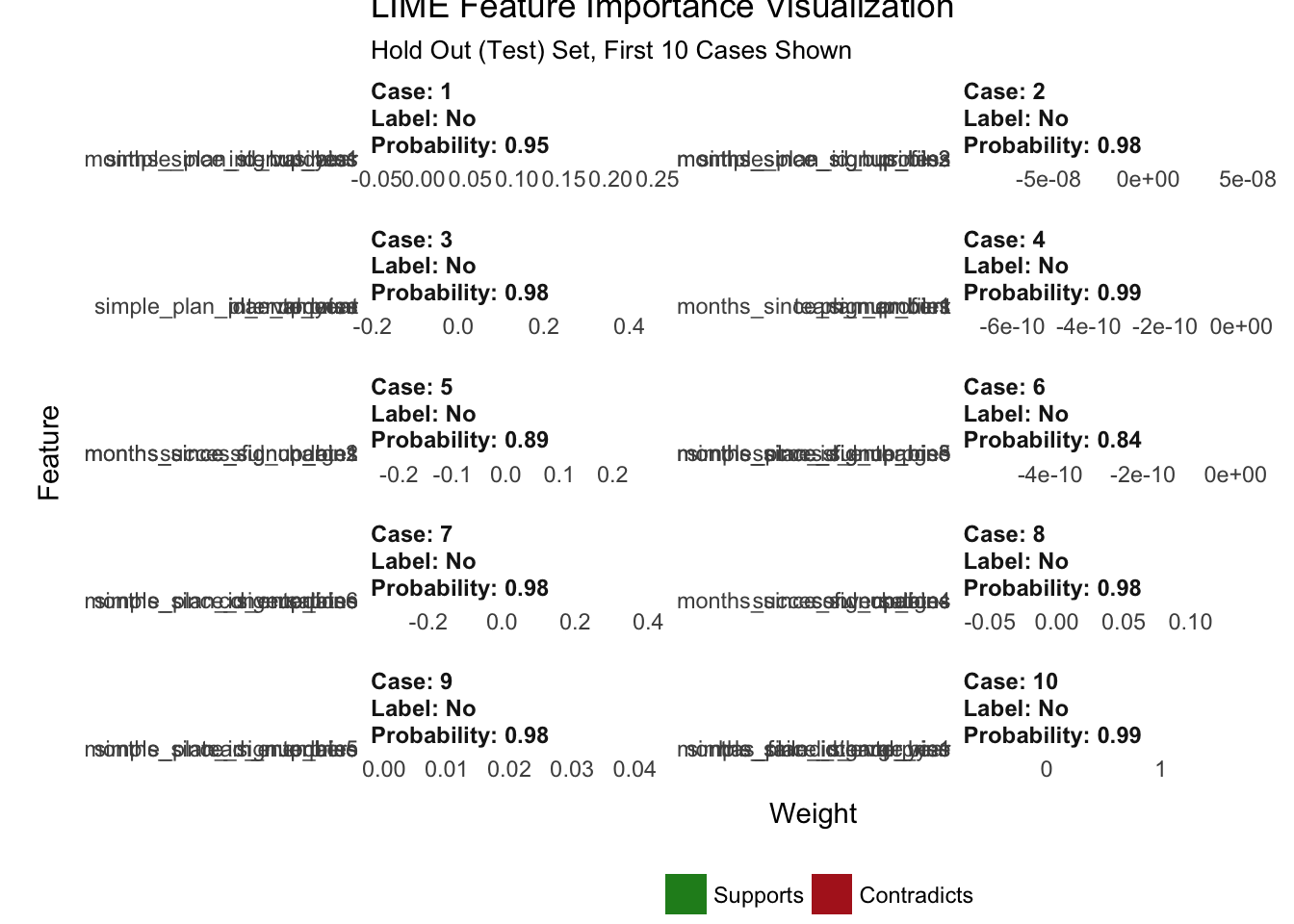

Another excellent visualization can be performed using plot_explanations(), which produces a facetted heatmap of all case/label/feature combinations. It’s a more condensed version of plot_features(), but we need to be careful because it does not provide exact statistics and it makes it less easy to investigate binned features.

plot_explanations(explanation) +
    labs(title = "LIME Feature Importance Heatmap",
         subtitle = "Hold Out (Test) Set, First 10 Cases Shown")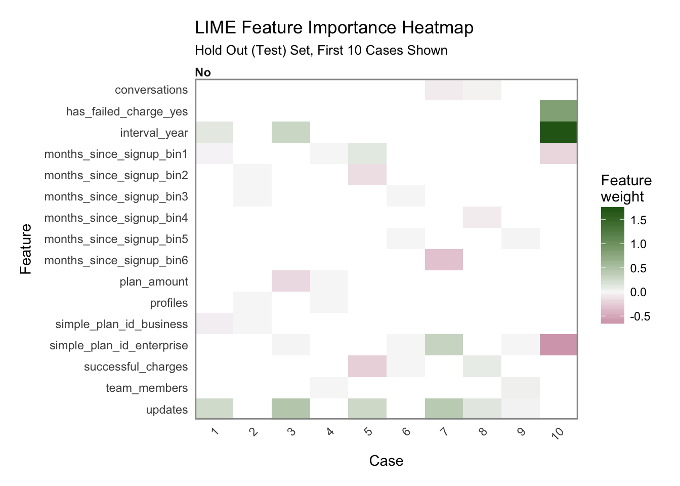

Checking explanations with correlation analysis

# Feature correlations to Churn
corr_analysis <- x_train_tbl %>%
  mutate(churned = y_train_vec) %>%
  correlate() %>%
  focus(churned) %>%
  rename(feature = rowname) %>%
  arrange(abs(churned)) %>%
  mutate(feature = as_factor(feature)) 

corr_analysis

## # A tibble: 16 x 2
##                      feature      churned
##                       <fctr>        <dbl>
##  1 simple_plan_id_enterprise -0.003811565
##  2  months_since_signup_bin4 -0.005386576
##  3  months_since_signup_bin3  0.007203574
##  4  months_since_signup_bin2  0.011171815
##  5                   updates -0.012636411
##  6  months_since_signup_bin5 -0.014485731
##  7                  profiles -0.014986354
##  8     has_failed_charge_yes  0.024346626
##  9               plan_amount -0.026337084
## 10  months_since_signup_bin6 -0.028114759
## 11   simple_plan_id_business -0.028392391
## 12  months_since_signup_bin1  0.028851225
## 13              team_members -0.030647368
## 14             conversations  0.030742660
## 15             interval_year -0.049423370
## 16        successful_charges -0.058451465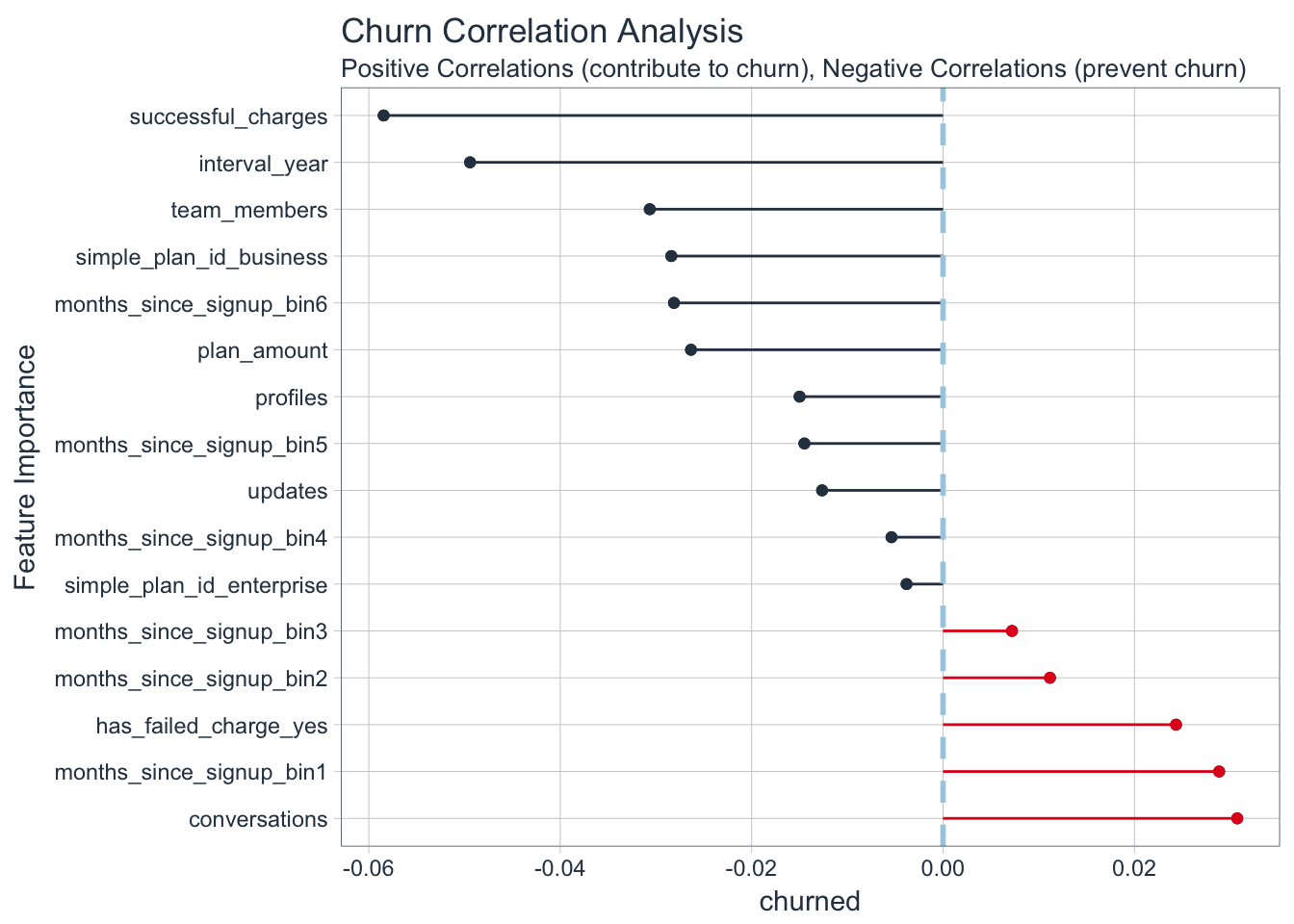

Notice that the correlation for each individual feature is quite small. Customers that have refunded charges and helpscout conversations are naturally more likely to churn. Subscriptions that have more successful charges and yearly subscriptions are less likely to churn.

That’s it for now!